Monopolist's Pricing and Output Decisions in Two Markets

The assignment is about a monopolist who must decide how to price and allocate product output between two geographic markets separated by a national border. The demand functions are Q1 = 30 - 2P1 and Q2 = 24 - P2, and the total cost is C = 5 + 2(Q1 + Q2). The monopolist's goal is to maximize profits under two conditions: (a) no arbitrage is possible, and (b) the border is opened to free trade and arbitrage. In condition (a), the firm can charge different prices in each market, and it is found that P1 = 8.5, Q1 = 13, and Q2 = 11, resulting in total profits of $200.5. In condition (b), the firm must charge a single price in both markets, and it is found that P = 10, Q = 24, and total profits are $187.

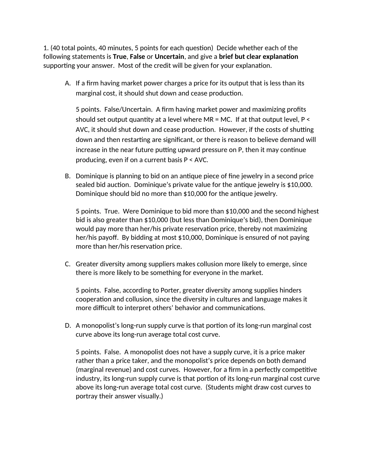
1. (40 total points, 40 minutes, 5 points for each question) Decide whether each of the
following statements is True, False or Uncertain, and give a brief but clear explanation
supporting your answer. Most of the credit will be given for your explanation.
A. If a firm having market power charges a price for its output that is less than its
marginal cost, it should shut down and cease production.
5 points. False/Uncertain. A firm having market power and maximizing profits
should set output quantity at a level where MR = MC. If at that output level, P <
AVC, it should shut down and cease production. However, if the costs of shutting
down and then restarting are significant, or there is reason to believe demand will
increase in the near future putting upward pressure on P, then it may continue
producing, even if on a current basis P < AVC.
B. Dominique is planning to bid on an antique piece of fine jewelry in a second price
sealed bid auction. Dominique’s private value for the antique jewelry is $10,000.
Dominique should bid no more than $10,000 for the antique jewelry.
5 points. True. Were Dominique to bid more than $10,000 and the second highest
bid is also greater than $10,000 (but less than Dominique’s bid), then Dominique
would pay more than her/his private reservation price, thereby not maximizing
her/his payoff. By bidding at most $10,000, Dominique is ensured of not paying
more than her/his reservation price.
C. Greater diversity among suppliers makes collusion more likely to emerge, since
there is more likely to be something for everyone in the market.
5 points. False, according to Porter, greater diversity among supplies hinders
cooperation and collusion, since the diversity in cultures and language makes it
more difficult to interpret others’ behavior and communications.
D. A monopolist’s long-run supply curve is that portion of its long-run marginal cost
curve above its long-run average total cost curve.
5 points. False. A monopolist does not have a supply curve, it is a price maker
rather than a price taker, and the monopolist’s price depends on both demand
(marginal revenue) and cost curves. However, for a firm in a perfectly competitive
industry, its long-run supply curve is that portion of its long-run marginal cost curve
above its long-run average total cost curve. (Students might draw cost curves to
portray their answer visually.)

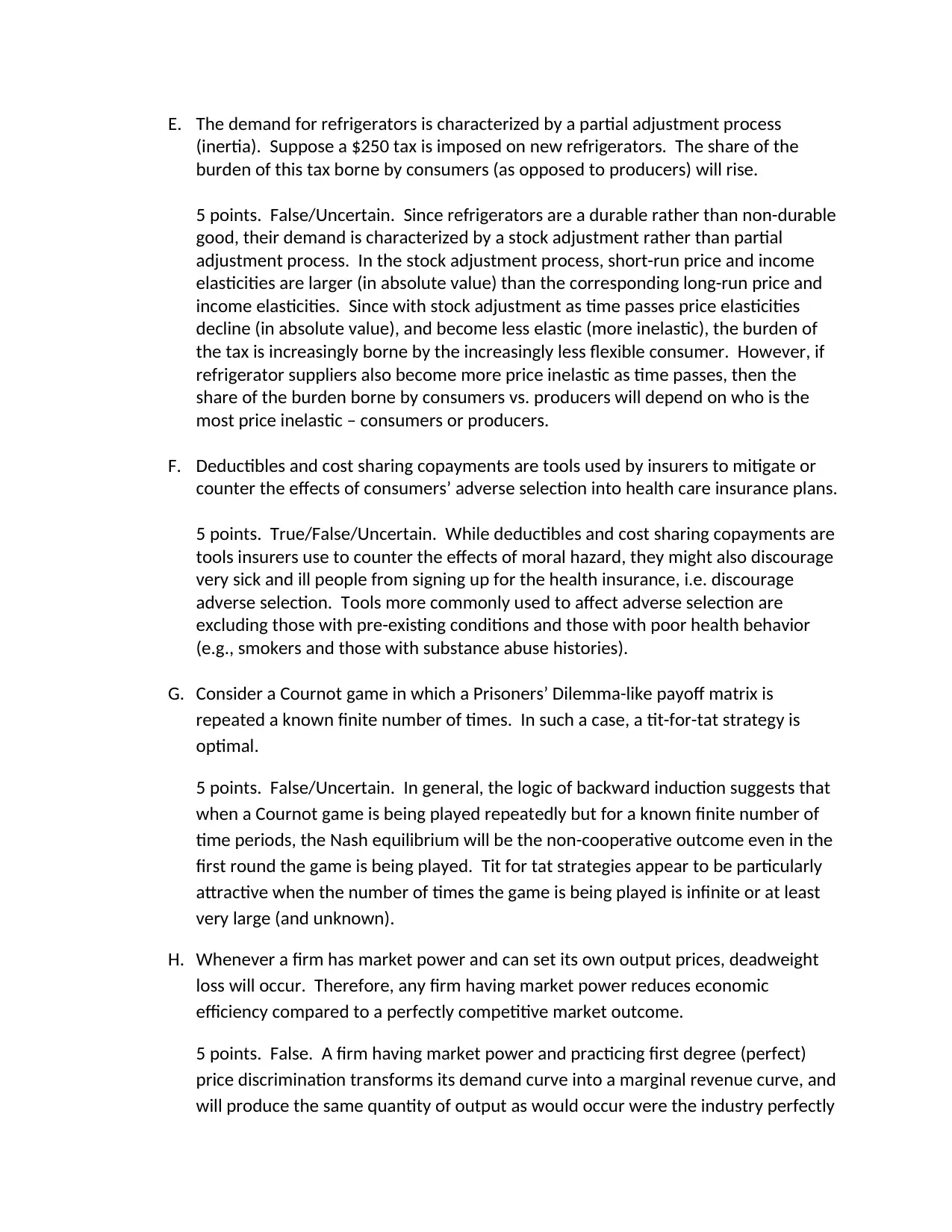
E. The demand for refrigerators is characterized by a partial adjustment process
(inertia). Suppose a $250 tax is imposed on new refrigerators. The share of the
burden of this tax borne by consumers (as opposed to producers) will rise.
5 points. False/Uncertain. Since refrigerators are a durable rather than non-durable
good, their demand is characterized by a stock adjustment rather than partial
adjustment process. In the stock adjustment process, short-run price and income
elasticities are larger (in absolute value) than the corresponding long-run price and
income elasticities. Since with stock adjustment as time passes price elasticities
decline (in absolute value), and become less elastic (more inelastic), the burden of
the tax is increasingly borne by the increasingly less flexible consumer. However, if
refrigerator suppliers also become more price inelastic as time passes, then the
share of the burden borne by consumers vs. producers will depend on who is the
most price inelastic – consumers or producers.
F. Deductibles and cost sharing copayments are tools used by insurers to mitigate or
counter the effects of consumers’ adverse selection into health care insurance plans.
5 points. True/False/Uncertain. While deductibles and cost sharing copayments are
tools insurers use to counter the effects of moral hazard, they might also discourage
very sick and ill people from signing up for the health insurance, i.e. discourage
adverse selection. Tools more commonly used to affect adverse selection are
excluding those with pre-existing conditions and those with poor health behavior
(e.g., smokers and those with substance abuse histories).
G. Consider a Cournot game in which a Prisoners’ Dilemma-like payoff matrix is
repeated a known finite number of times. In such a case, a tit-for-tat strategy is
optimal.
5 points. False/Uncertain. In general, the logic of backward induction suggests that
when a Cournot game is being played repeatedly but for a known finite number of
time periods, the Nash equilibrium will be the non-cooperative outcome even in the
first round the game is being played. Tit for tat strategies appear to be particularly
attractive when the number of times the game is being played is infinite or at least
very large (and unknown).
H. Whenever a firm has market power and can set its own output prices, deadweight
loss will occur. Therefore, any firm having market power reduces economic
efficiency compared to a perfectly competitive market outcome.
5 points. False. A firm having market power and practicing first degree (perfect)
price discrimination transforms its demand curve into a marginal revenue curve, and
will produce the same quantity of output as would occur were the industry perfectly

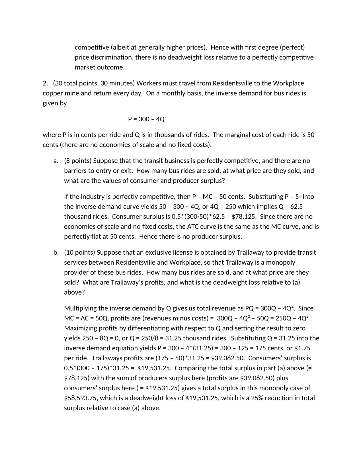
competitive (albeit at generally higher prices). Hence with first degree (perfect)
price discrimination, there is no deadweight loss relative to a perfectly competitive
market outcome.
2. (30 total points, 30 minutes) Workers must travel from Residentsville to the Workplace
copper mine and return every day. On a monthly basis, the inverse demand for bus rides is
given by
P = 300 – 4Q
where P is in cents per ride and Q is in thousands of rides. The marginal cost of each ride is 50
cents (there are no economies of scale and no fixed costs).
a. (8 points) Suppose that the transit business is perfectly competitive, and there are no
barriers to entry or exit. How many bus rides are sold, at what price are they sold, and
what are the values of consumer and producer surplus?
If the industry is perfectly competitive, then P = MC = 50 cents. Substituting P = 5- into
the inverse demand curve yields 50 = 300 – 4Q, or 4Q = 250 which implies Q = 62.5
thousand rides. Consumer surplus is 0.5*(300-50)*62.5 = $78,125. Since there are no
economies of scale and no fixed costs, the ATC curve is the same as the MC curve, and is
perfectly flat at 50 cents. Hence there is no producer surplus.
b. (10 points) Suppose that an exclusive license is obtained by Trailaway to provide transit
services between Residentsville and Workplace, so that Trailaway is a monopoly
provider of these bus rides. How many bus rides are sold, and at what price are they
sold? What are Trailaway’s profits, and what is the deadweight loss relative to (a)
above?
Multiplying the inverse demand by Q gives us total revenue as PQ = 300Q – 4Q2. Since
MC = AC = 50Q, profits are (revenues minus costs) = 300Q – 4Q2 – 50Q = 250Q – 4Q2 .
Maximizing profits by differentiating with respect to Q and setting the result to zero
yields 250 – 8Q = 0, or Q = 250/8 = 31.25 thousand rides. Substituting Q = 31.25 into the
inverse demand equation yields P = 300 – 4*(31.25) = 300 – 125 = 175 cents, or $1.75
per ride. Trailaways profits are (175 – 50)*31.25 = $39,062.50. Consumers’ surplus is
0.5*(300 – 175)*31.25 = $19,531.25. Comparing the total surplus in part (a) above (=
$78,125) with the sum of producers surplus here (profits are $39,062.50) plus
consumers’ surplus here ( = $19,531.25) gives a total surplus in this monopoly case of
$58,593.75, which is a deadweight loss of $19,531.25, which is a 25% reduction in total
surplus relative to case (a) above.

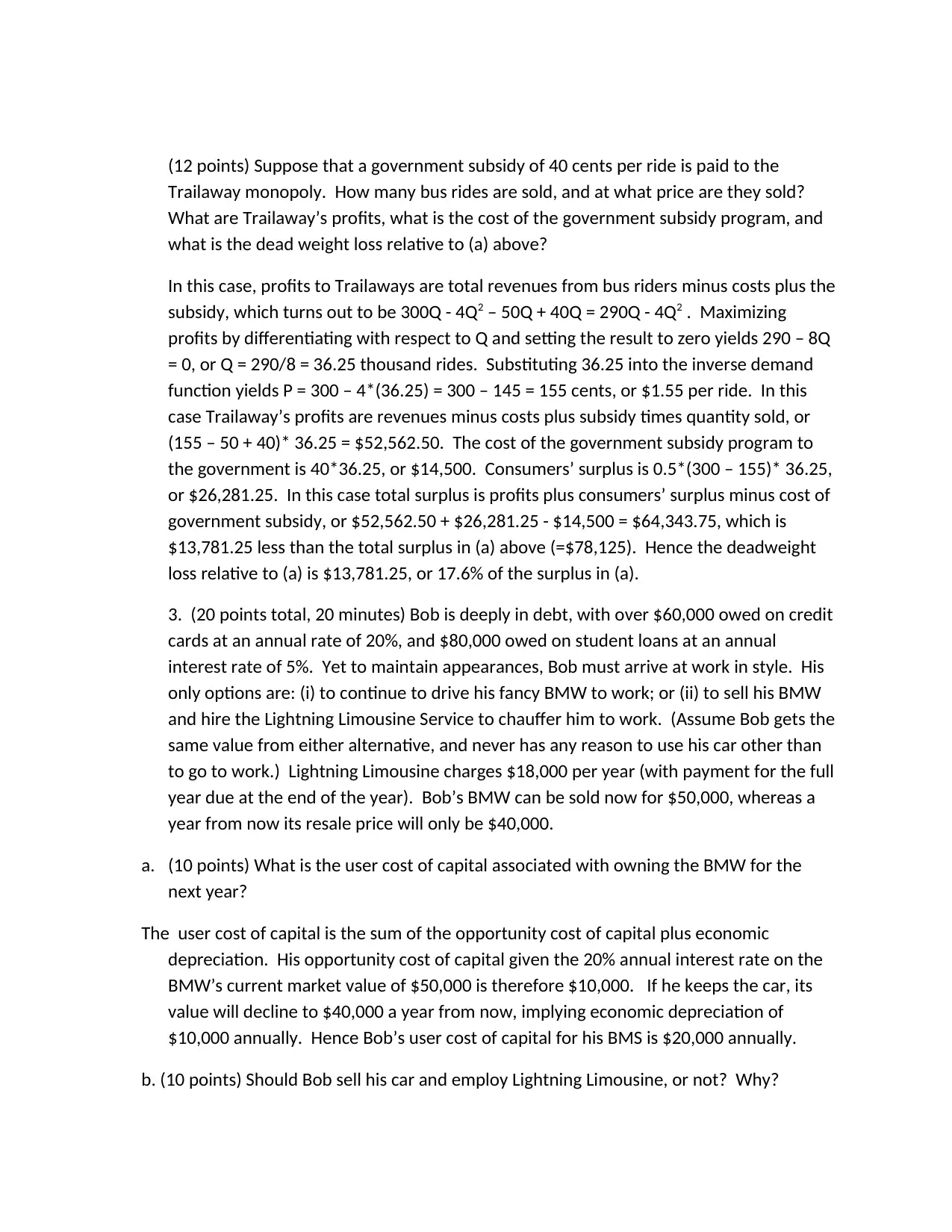
(12 points) Suppose that a government subsidy of 40 cents per ride is paid to the
Trailaway monopoly. How many bus rides are sold, and at what price are they sold?
What are Trailaway’s profits, what is the cost of the government subsidy program, and
what is the dead weight loss relative to (a) above?
In this case, profits to Trailaways are total revenues from bus riders minus costs plus the
subsidy, which turns out to be 300Q - 4Q2 – 50Q + 40Q = 290Q - 4Q2 . Maximizing
profits by differentiating with respect to Q and setting the result to zero yields 290 – 8Q
= 0, or Q = 290/8 = 36.25 thousand rides. Substituting 36.25 into the inverse demand
function yields P = 300 – 4*(36.25) = 300 – 145 = 155 cents, or $1.55 per ride. In this
case Trailaway’s profits are revenues minus costs plus subsidy times quantity sold, or
(155 – 50 + 40)* 36.25 = $52,562.50. The cost of the government subsidy program to
the government is 40*36.25, or $14,500. Consumers’ surplus is 0.5*(300 – 155)* 36.25,
or $26,281.25. In this case total surplus is profits plus consumers’ surplus minus cost of
government subsidy, or $52,562.50 + $26,281.25 - $14,500 = $64,343.75, which is
$13,781.25 less than the total surplus in (a) above (=$78,125). Hence the deadweight
loss relative to (a) is $13,781.25, or 17.6% of the surplus in (a).
3. (20 points total, 20 minutes) Bob is deeply in debt, with over $60,000 owed on credit
cards at an annual rate of 20%, and $80,000 owed on student loans at an annual
interest rate of 5%. Yet to maintain appearances, Bob must arrive at work in style. His
only options are: (i) to continue to drive his fancy BMW to work; or (ii) to sell his BMW
and hire the Lightning Limousine Service to chauffer him to work. (Assume Bob gets the
same value from either alternative, and never has any reason to use his car other than
to go to work.) Lightning Limousine charges $18,000 per year (with payment for the full
year due at the end of the year). Bob’s BMW can be sold now for $50,000, whereas a
year from now its resale price will only be $40,000.
a. (10 points) What is the user cost of capital associated with owning the BMW for the
next year?
The user cost of capital is the sum of the opportunity cost of capital plus economic
depreciation. His opportunity cost of capital given the 20% annual interest rate on the
BMW’s current market value of $50,000 is therefore $10,000. If he keeps the car, its
value will decline to $40,000 a year from now, implying economic depreciation of
$10,000 annually. Hence Bob’s user cost of capital for his BMS is $20,000 annually.
b. (10 points) Should Bob sell his car and employ Lightning Limousine, or not? Why?

Since Lightning Limousine charges only $18,000 per year with payment for the full year
due at the end of the year, it is less costly for Bob to contract with Lightning Limousine to
chauffer him to work and sell his BMS (a total cost of $18,000 annually) than it is to
continue to own his car and drive to work (whose total annual user cost of capital would be
$20,000). Bob should bite the dust, hold his chin high, sell his BMS, and enjoy Lightning
Limousine services.
4. (30 total points, 30 minutes) Suppose that two identical firms produce widgets and that they
are the only firms in the market. Their total costs are given by C1 = 30Q1 and C2 = 30Q2, where
Q1 is the output of Firm 1 and Q2 is the output of Firm 2. Price is determined by the following
inverse demand curve:
P = 150 – Q, where Q ≡ Q1 + Q2.
a. (8 points) Find the Cournot-Nash equilibrium. Calculate the profits of each firm at this
equilibrium.
Substituting Q ≡ Q1 + Q2 into the inverse demand equation and multiplying the result by Q1
yields firm 1’s total revenues. Taking into account Firm 1’s costs yields Firm 1’s profits as
150*Q1 – Q12 – Q1*Q2 – 30*Q1. Differentiating these profits of Firm 1 with respect to Q1 and
setting the expression to zero yields 120 – 2*Q1 – Q2 = 0, which gives us Firm 1’s reaction
function as Q1 = 60 – 0.5*Q2. Since Firm 2 faces the same inverse demand function as Firm 1
and has the same costs per unit of its output as does Firm 1, Firm 2’s reaction function is
symmetric, and is Q2 = 60 – 0.5*Q1. These two reaction functions give us two equations in two
unknowns, which we can solve as follows: Q1 = 60 – 0.5*(60 – 0.5*Q1) = 60 – 30 + 0.25*Q1,
which implies that 0.75*Q1 = 30, or Q1 = 40. Since Firm 2 has a symmetric reaction function, it is
also the case that Q2 = 40. (Alternatively substitute Q1 = 40 into Firm 2’s reaction function
above, yielding Q2 – 60 – 05*40 = 60 – 20 = 40.) Given symmetric reaction functions, that they
have the same costs and face the same market demand function, the profits for each of the two
firms is total revenues minus total costs, or 70*40 – 30*40 = $1600 for both firms.
b. (8 points) Suppose the two firms form a cartel to maximize joint profits, which they
agree to share equally. How many widgets will each firm produce? Calculate each
firm’s profits.
To get the cartel’s total revenues, multiply the inverse demand equation by Q. To get the
cartel’s profits, subtract 30*Q from the cartel’s total revenues. This yields the cartel’s total
profits as P*Q = 150 *Q– Q2 – 30Q = 120Q – Q2. Differentiating this profit function with
respect to Q and setting the expression equal to zero yields 120 – 2*Q = 0, which implies that Q
= 60. Substituting Q = 60 into the inverse demand function yields P = 150 – 60 = 90. Assuming

the two cartel produce equal amounts of 30 widgets, each firm’s profits in this cartel situation is
90*30 – 30*30 = 60*30 = $1800. Note that profits for the cartel at $1800 each are larger than
in the Cournot case, where profits are $1600 for each firm. The increased profits result from
the cartel effectively restricting cartel output, driving up industry price.
c. (6 points) Suppose Firm 1 were the only firm in the industry. How would the market
output and Firm 1’s profits differ from that found in part (b) above? Why?
Since the cartel is effectively acting as a monopolist maximizing joint profits for the cartel, if in
fact the cartel were transformed from a duopoly to a monopoly there would be no impact on
output, which would remain at 60 for the monopolist, and given the industry inverse demand
function, the market price would remain at $90. Given constant average and marginal costs of
$30, the monopolist’s profits would now be $60*60 = $3600, which is precisely the same as the
total profits of the two-firm cartel in (b) above.
d. (8 points) Returning to the duopoly of part (b), Firm 2 knows that Firm 1 will abide by
the agreement, but Firm 2 decides to take advantage of Firm 1’s credible faithful
commitment by increasing Firm 2’s production. How many widgets will Firm 2 produce?
What will be each firm’s profits?
This transforms the Cournot duopoly problem in (b) above into the same as the first-mover
advantage game we called the Stackleberg game. In particular, if Firm 2 knows that Firm 1 will
be faithful to its reaction function, then Firm 2 uses that information in making its decision to
“cheat” and take advantage of Firm 1’s fidelity. Specifically, since Firm 2 knows that Q1 = 30,
Firm 2 can substitute this into its inverse demand function, changing P = 150 – Q1 – Q2 to
P = 150 – 30 – Q2 = 120 – Q2. Multiplying this last equation by Q2 to get Firm 2’s total revenues
and then subtracting Firm 2’s total costs gives us Firm 2’s profits as being equal to
(120 – Q2)*Q2 – 30Q2 = 120*Q2 – Q22 – 30Q2. Differentiating this profit function with respect to
Q2 and setting the result equal to zero yields 120 – 2*Q2 – 30 = 0 which implies that 2*Q2 = 90,
or Q2 = 45. Notice that knowing that Firm 1 will produce 30, Firm 2 increases its output, from
instead of the Cournot agreed upon output for each firm at 30, to 45. As a result, substituting
Q2 = 45 into Firm 2’s inverse demand function (see six lines above), we have that P = 120 – Q2 =
120 – 45 = 75. In this case, both Firm 1’s and Firm 2’s profits will be total revenues minus total
costs, but since Firm 2 is producing more, taking advantage of Firm 1’s known fidelity, we have
that for Firm 2, profits are (75 – 30)*45 = $2025, whereas for Firm 1, profits are (75 – 30)*30 =
$1350. Notice that while in this case total profits of Firms 1 and 2 at $3375 ($2025 + $1350) are
larger than in the Cournot case (a) above (where each firm had profits of $1600), now Firm 2
has increased its profits from $1600 to $2025, all at the expense of the faithful Firm 1, whose
profits have now fallen from $1800 to $1350.
5. (16 total points, 16 minutes) The United States and Russia are considering policies to open or
close their import markets. Suppose the payoff matrix has payoffs of x,y, where where x is the
payoff to the United States and y is the payoff to Russia:

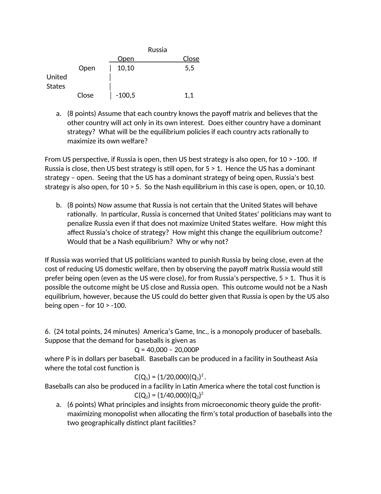
Russia
Open Close
Open | 10,10 5,5
United │
States │
Close │ -100,5 1,1
a. (8 points) Assume that each country knows the payoff matrix and believes that the
other country will act only in its own interest. Does either country have a dominant
strategy? What will be the equilibrium policies if each country acts rationally to
maximize its own welfare?
From US perspective, if Russia is open, then US best strategy is also open, for 10 > -100. If
Russia is close, then US best strategy is still open, for 5 > 1. Hence the US has a dominant
strategy – open. Seeing that the US has a dominant strategy of being open, Russia’s best
strategy is also open, for 10 > 5. So the Nash equilibrium in this case is open, open, or 10,10.
b. (8 points) Now assume that Russia is not certain that the United States will behave
rationally. In particular, Russia is concerned that United States’ politicians may want to
penalize Russia even if that does not maximize United States welfare. How might this
affect Russia’s choice of strategy? How might this change the equilibrium outcome?
Would that be a Nash equilibrium? Why or why not?
If Russia was worried that US politicians wanted to punish Russia by being close, even at the
cost of reducing US domestic welfare, then by observing the payoff matrix Russia would still
prefer being open (even as the US were close), for from Russia’s perspective, 5 > 1. Thus it is
possible the outcome might be US close and Russia open. This outcome would not be a Nash
equilibrium, however, because the US could do better given that Russia is open by the US also
being open – for 10 > -100.
6. (24 total points, 24 minutes) America’s Game, Inc., is a monopoly producer of baseballs.
Suppose that the demand for baseballs is given as
Q = 40,000 – 20,000P
where P is in dollars per baseball. Baseballs can be produced in a facility in Southeast Asia
where the total cost function is
C(Q1) = (1/20,000)(Q1)2 .
Baseballs can also be produced in a facility in Latin America where the total cost function is
C(Q2) = (1/40,000)(Q2)2
a. (6 points) What principles and insights from microeconomic theory guide the profit-
maximizing monopolist when allocating the firm’s total production of baseballs into the
two geographically distinct plant facilities?

What we learned from our multiplant monopolist discussion is that if a firm decides to produce
simultaneously at multiplant locations, and if there are no transport or transactions costs, the
multiplant monopolist will always allocate production among the various plants so that their
marginal costs are identical. If marginal costs were not identical, the multiplant monopolist
could produce the same total multiplant output by increasing output at the lower marginal cost
plants and decreasing output at the higher marginal cost plants, thereby reducing total costs
over the multiple plants. When one combines producing at that output at which MR = MC =
MC1 = MC2 = MC total, we obtain the solution for the total output over the two plants.
b. (12 points) Illustrate graphically the monopolist’s problem. What is the monopolist’s
optimal total production level over both production facilities, and what is the optimal
production allocation for baseballs in the two distinct production facilities? Is any
output produced in the Southeast Asia production facility, given that its cost curve is
higher than that for Latin America, at all common output levels? Why or why not?
Note that MC1 = 2*Q1/20,000, so Q1 = MC1*10,000; Since MC2 = Q2/20,000, Q2 = MC2*20,000.
Hence Q = Q1 + Q2 = MC1*10,000 + MC2*20,000. But since MC1 must = MC2 = MCtotal, it follows
that Q = (10,000 + 20,000)*MCtotal which implies that MCtotal. = Q/30,000. These results reflect
the equal MC restriction across plants that must be satisfied. So in the graph we then must find
that level of Q at which MR = MCtotal. So now let’s work on the MR = MC relationship.
In order to set marginal revenue equal to MCtotal. we first need to transform the demand
function with Q depending on P into an inverse demand function with P depending on Q. Since

Q = 40,000 – 20,000*P, we obtain the inverse demand function P = 2 – (Q/20,000). Multiplying
by Q to get total revenues, we have P*Q = 2*Q – (Q2/20,000). Marginal revenue is therefore
the partial derivative of total revenues with respect to Q. This turns out to give us MR = 2 –
(2*Q/20,000) = 2 – Q/10,000 which in turn can be written as MR = 2 – (Q1 + Q2)/10,000 which
implies that MR = 2 – Q/10,000. The various marginal cost curves and the marginal revenue
curve are graphed above. As can be seen there, the optimal total firm output is 15,000, with
Southeast Asia output Q1 allocated 5,000 units, and Latin America output Q2 allocated 10,000
units. Although at any common level of output marginal costs in Southeast Asia are greater
than in Latin America, when output in Latin America is increased until its marginal cost just
equals the marginal cost of the first unit produced in Southeast Asia, output from Southeast
Asia kicks in, and thereafter while more output is always produced in Latin America than in
Southeast Asia, both plants are utilized up to the point where their marginal costs are
equalized.
c. (6 points) What is the optimal price of baseballs (show all calculations)? How many are
produced in Southeast Asia? How many are produced in Latin America? What are total
profits to America’s Game, Inc.?
To solve this analytically rather than graphically, let’s use the MCtotal and MR relationships in
boldface in part (b) above, and set them equal to each other, and then solve for Q. Hence,
Q/30,000 = 2 – Q/10,000. We can re-write the right hand side of this as (60,000 – 3Q)/30,000.
Since we now have a common denominator of 30,000, we just set the numerators equal to
each other, giving us Q = 60,000 – 3Q, implying 4Q = 60,000, or Q = Q1 + Q2 = 15,000. To find
the optimal allocation of Q to the Southeast Asian and Latin American plants, note that since
MC1 = 2*Q1/20,000 and MC2 = Q2/20,000, we can set them equal to each other, and since they
have the same 20,000 denominator, we can just set their numerators equal to each other,
yielding 2*Q1 = Q2. Since from above (see immediate boldface above) Q1 + Q2 = 15,000, we have
that Q1 + Q2 = Q1 + 2*Q1 = 3*Q1 = 15,000, implying that Q1 = 5,000 and Q2 = 10,000.
Regarding price, since earlier in part (b) above we established that the inverse demand function
was P = 2 – (Q/20,000), we now have that P = 2 – (15,000/20,000) = $1.25 per baseball. Total
revenues are therefore $1.25*15,000 = $18,750. Substituting Q1 = 5,000 and Q2 = 10,000 into
the total cost functions C(Q1) = (1/20,000)(Q1)2 and C(Q2) = (1/40,000)(Q2)2 , we have for Plant 1,
C1 = 25,000,000/20,000 = $1,250, and C2 = 100,000,000/40,000 = $2,500. Total profits to
America’s Game, Inc. are therefore revenues minus costs, or $18,750 - $1,250 - $2,500 =
$15,000.
7. (20 total points, 20 minutes) A monopolist must decide how to price in two markets and
allocate product output between them. The markets are separated geographically (being either
side of a national border). Demands in the two markets are as follows:
Q1 = 30 – 2P1 and Q2 = 24 – P2.

The monopolists total cost are C = 5 + 2(Q1 + Q2).
What are the prices charged, total product shipped to each market, and total profits to the
monopolist under the following two conditions?
a. (12 points) The markets are separated, and no arbitrage is possible (the firm can ship to
both markets, but there is no other trade in the particular product)?
If no arbitrage is possible, the firm can charge different prices in the two markets, and not
have to worry about reselling. First we transform the demand functions into inverse
demand fuctions. Since Q1 = 30 – 2P1, P1 = 15 – 0.5*Q1. Similarly, since Q2 = 24 – P2., it
follows that P2 = 24 – Q2. Given the cost information above, profits from sales in both
markets are therefore written as revenues in both markets minus costs in both markets:
(15 – 0.5*Q1)*Q1 + (24 – Q2)*Q2 – 5 – 2*(Q1 + Q2). Multiplying these out and collecting
terms yields profits as 15*Q1 – 0.5*Q12 + 24*Q2 – Q22 – 5 – 2*Q1 – 2*Q2. Differentiating this
with respect to Q1 and setting the result equal to zero yields 15 – Q1 – 2 = 0 which implies
that Q1 = 13. Differentiating with respect to Q2 and setting the result equal to zero yields 24
– 2*Q2 – 2 = 0 which implies 2*Q2 = 22, or Q2 = 11. Substituting these outputs into the
inverse demand functions P1 = 15 – 0.5*Q1 and P2 = 24 – Q2, we have P1 = 15 – 0.5*13 = 8.5,
and P2 = 24 – 11 = 13. Total revenues are 110.5 + 143 = 253.5, total costs are 5 + 2*(Q1 + Q2)
= 5 + 2*(13 + 11) = 5 + 48 = 53. So total profits are 253.5 – 53 = 200.5.
b. (8 points) The border is opened to free trade and possible arbitrage.
If there is only one market with arbitrage permitted, then a single price will prevail in the two
markets. In that case (since P1 = P2) Q = Q1 + Q5= 30 – 2*P + 24 – P = 54 – 3*P, which implies
that P = 18 – (1/3)*Q. In this case, total revenues = P*Q = 18Q – (1/3)*Q2, total costs are 5 +
2*Q, so that profits are 16Q – (1/3)Q2 – 5. Differentiating this profit function with respect to Q
and setting the result equal to zero results in 16 – (2/3)*Q = 0, which implies (2/3)*Q = 16, or Q
= 24. Substituting Q = 24 into the inverse demand function P = 18 – (1/3)*Q => P = 18 –
(1/3)*24 => P = 18 – 8 = 10. Notice that Q = 24 is identical to the total output the monopolist
produced and sold when arbitrage was not possible, but price discrimination was feasible. This
is a mathematical result derived from demand curves being linear, and cost functions identical –
the same total output will be produced and sold by the monopolist regardless of whether price
discrimination is feasible or not. However, in this particular case where arbitrage is possible
and there is a single uniform price in the two geographical regions, the uniform price will be 10
(in between the 8.5 and 13 prices when price discrimination is feasible), so that the firm’s
profits will be 10*24 – 5 – 2*(24) = 187. Of the total output of 24 at P = 10, Q1 = 30 – 20 = 10,
and Q2 = 24 – 10 = 14. Two other comments. Note that global output is identical at 24
regardless of whether price discrimination or uniform pricing occurs. This is a mathematical
result that occurs when the inverse demand curves for each geographic area are linear, and
marginal costs are constant and equal across geographies. Second, despite producing the same
total global output, note that the firm’s total profits are larger under price discrimination than

under uniform pricing. This reflects the fact that price discrimination allows the firm to convert
some consumers’ surplus under uniform pricing into producer’s surplus under price
discrimination.