Probability and Statistics

This document discusses various probability and statistics concepts such as probability calculations, association rules, frequency plots, gamma distribution, and more. It also includes R code examples and explanations. The subject is Probability and Statistics.

1
(a)
The probability that you are detained for further testing = 0.20.
(b)
The probability that any given driver will be detained = 0.8 ×0.12 +0.2 ×0.88 = 0.096 +0.176 = 0.272.
(c)
P ( Drinking | Detained) = (0.8 ×0.12)/0.272 = 0.353.
(d)
P ( Drinking | Released) = (0.12 ×0.2)/(0.8 ×0.12 +0.88 ×0.8) = 0.024/0.728 = 0.033
2
(a)
The support for Rule 1, supp (S) = 5/6 = 0.833.
The confidence for Rule 1, conf (S => M) = supp (S ∪ M) / supp (S). Now supp (S ∪ M) = 3/6 = 0.5. Therefore,
conf (S => M) = (0.5/0.833) = 0.6.
(b)
The support for Rule 2, supp (M) = 4/6 = 0.667.
The confidence for Rule 2, conf (M => S) = supp (S ∪ M) / supp (M). Now supp (S ∪ M) = 3/6 = 0.5. Therefore,
conf (M => s) = (0.5/0.667) = 0.75.
(c)
The lift for Rule 1, lift (M = > S) = supp (S ∪ M) / (supp (M) × supp (S)) = 0.5/(0.833 × 0.667) = 0.899 . Since
the lift is also same for lift (S = > M). We will use the confidence to determine which is more associated. As the
conf (M => s) is greater so the Rule 2 is a better association.
1

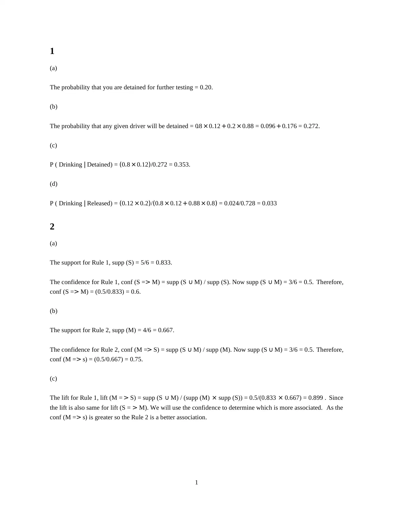
Figure 1: Figure to represent support for the first 8 items
3
(a)
R Code:
data(Groceries) Groceries.items <- Groceries[Groceries %in% "bags"]
itemFrequencyPlot(Groceries.items[, 1:8], population = Groceries[, 1:8])
The required frequency plot for the first 8 items refer figure (1).
(b)
R Code:
data(Groceries) Groceries.items <- Groceries[Groceries %in% "bags"]
itemFrequencyPlot(Groceries.items, population = Groceries, support = 0.05, lift = TRUE, horiz = FALSE)
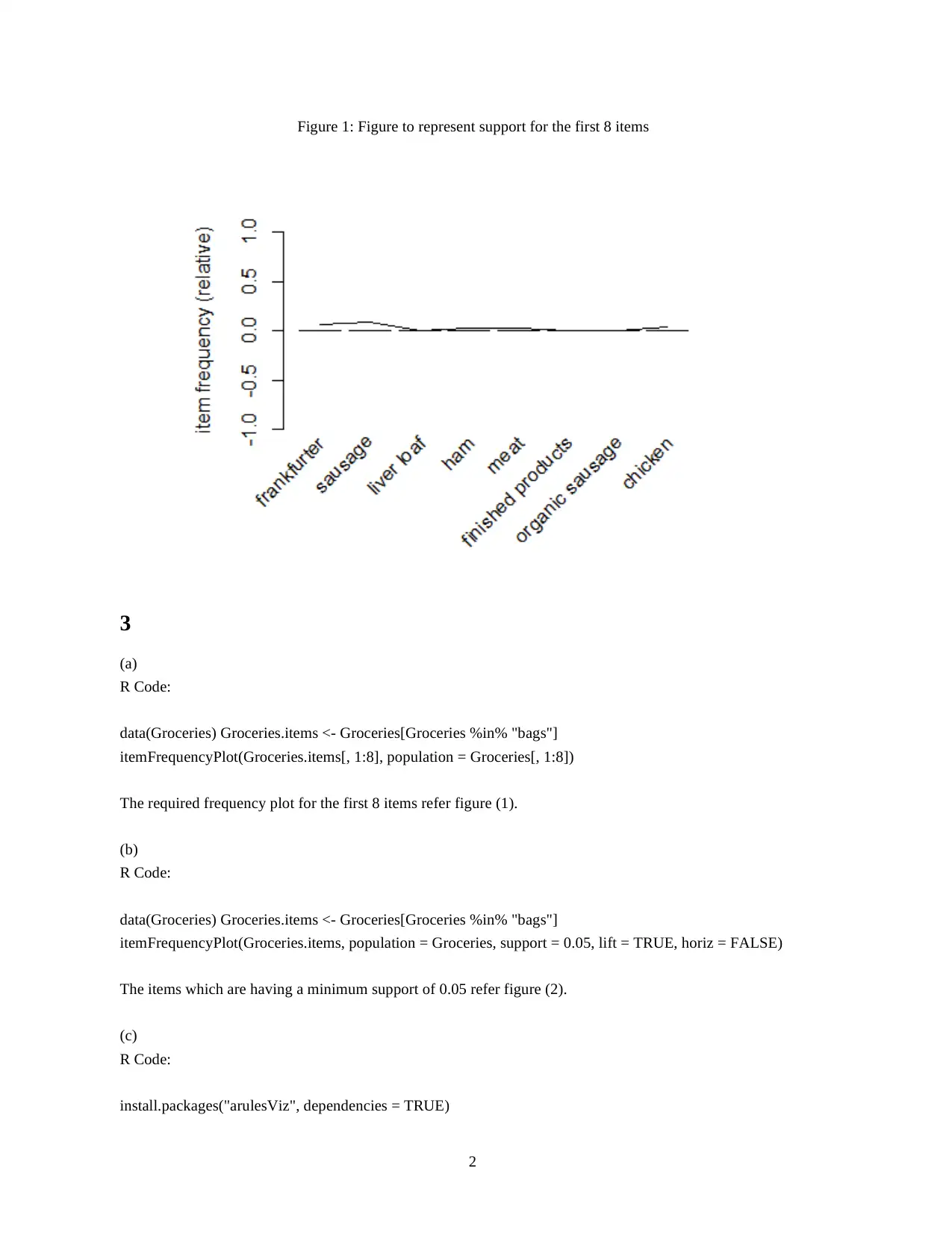
The items which are having a minimum support of 0.05 refer figure (2).
(c)
R Code:
install.packages("arulesViz", dependencies = TRUE)
2

Figure 2: Items having minimum support of 0.05
library(arulesViz)
But I am getting this error
Error in plot.associations(rules) : Needed package ’arulesViz’ not installed or loaded!
The package which is used to install in R is not working as I have tried all other means to draw the bubble chart.
4
(a)
f(t) = dF (T )
dt = d
dt 1 − 1
(1+t)α = α
(1+t)α+1 .
(b)
E(T ) =
Z ∞
0
t α
(1 +t)α+1 dt
let (1+t) = z, substituting this in to the equation,
E(T ) =
Z ∞
1
(z −1) α
zα+1 dz
3

E(T ) = α
Z ∞
1
(z−α −z−α−1)dz
E(T ) = α(−1
α − 1
−α +1 ) = 1
α −1
(c)
E(T 2) =
Z ∞
0
t2 α
(1 +t)α+1 dt
let (1+t) = z, substituting this in to the equation,
E(T 2) =
Z ∞
1
(z −1)2 α
zα+1 dz
E(T 2) = α
Z ∞
1
(z1−α −2z−α +z−α−1)dz
E(T 2) = α( −1
2 −α +2 1
1 −α + 1
α ) = 2
(2 − α)(1 − α) = 2
(α −2)(α −1)
V (T ) =E(T 2) − (E(T ))2 = 2
(α −2)(α −1) − ( 1
α −1 )2 = α
(α −1)2(α −2)
5
(a)
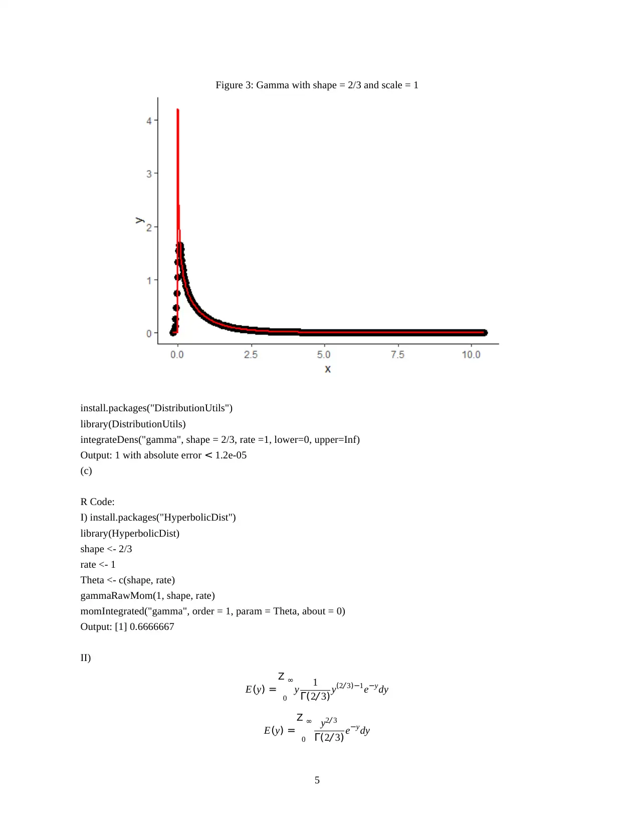
By taking x3 = y, we can reduce the f(x) in to
f (y) = 1
Γ(2/ 3) y(2/ 3)−1e−y
where k the shape parameter = 2/3 andθ the scale parameter = 1. Using this form in the R code we get the follow-
ing plot (3).
R Code:
library(ggplot2)
library(MASS)
# Generate gamma rvs
x <- rgamma(100000, shape = 2/3, rate = 1)
den <- density(x)
dat <- data.frame(x = den$x, y = den$y) # Plot using density points
ggplot(data = dat, aes(x = x, y = y)) + geom_point(size = 3) + geom_line(aes(x=dat$x, y=dgamma(dat$x, fit.params$ estimate[”shape”],
fit.params$estimate[”rate”])), color="red", size = 1) + theme_classic()
(b)
R Code:
4

Figure 3: Gamma with shape = 2/3 and scale = 1
install.packages("DistributionUtils")
library(DistributionUtils)
integrateDens("gamma", shape = 2/3, rate =1, lower=0, upper=Inf)
Output: 1 with absolute error < 1.2e-05
(c)
R Code:
I) install.packages("HyperbolicDist")
library(HyperbolicDist)
shape <- 2/3
rate <- 1
Theta <- c(shape, rate)
gammaRawMom(1, shape, rate)
momIntegrated("gamma", order = 1, param = Theta, about = 0)
Output: [1] 0.6666667
II)
E(y) =
Z ∞
0
y 1
Γ(2/ 3) y(2/ 3)−1e−ydy
E(y) =
Z ∞
0
y2/ 3
Γ(2/ 3) e−ydy
5

Now Mutipliying Γ(5/ 3) both numerator and denominator, we can write
E(y) =
Z ∞
0
y5/ 3−1
Γ(2/ 3) e−y Γ(5/ 3)
Γ(5/ 3) dy
E(y) = Γ(5/ 3)
Γ(2/ 3)
Z ∞
0
y5/ 3−1
Γ(5/ 3) e−ydy
E(y) = Γ(5/ 3)
Γ(2/ 3)
As, Z ∞
0
y5/ 3−1
Γ(5/ 3) e−ydy = 1
Therefore we can write,
E(y) = Γ(5/ 3)
Γ(2/ 3) = 2
3
Γ(2/ 3)
Γ(2/ 3) = 2
3 = 0.6666667
Thus, it is proved that the result of I and II are same.
(d)
R Code:
integrateDens("gamma",shape = 2/3, rate =1,lower=1.5,upper=Inf)
P(X > 1.5) i.e. the demand will exceed supply is 0.1247272 with absolute error < 1.8e-06.
(e)
R Code:
integrateDens("gamma",shape = 2/3, rate =1,lower=0.05,upper=1.5)
Probability that the company will be in a perilous financial position unless they sell at least 50 units of the product
in July is 0.7278908 with absolute error < 1.1e-05.
6
(a)
Probability is 0.2.
(b)
FX,Y (2000, 400) = 0.3 + 0.2 = 0.5.
(c)
6

P (X = 1600) = 0.55
P (X = 2000) = 0.30
P (X = 2400) = 0.15
(d)
P ( X + Y = 2400) occurs in two case when X = 2000 and Y = 400 or when X = 1600 and Y = 800. Therefore, P
( T = 2400) = P (X = 2000, Y = 400) + P (X = 1600, Y = 800) = 0.2 + 0.25 = 0.45. Like this we have to calculate
all other probabilities
t 2000 2400 2400 2800
fT (t) 0.30 0.45 0.2 0.05
(e)
E(T ) =2000 ×0.3 +2400 ×0.45 +2800 times0.2 +3200 ×0.05 = 2400
(f)
P ( 1600 | 400) = P(1600∩400)
P(400)
Now P (400) = 0.3 + 0.2 + 0.1 = 0.6
P ( 1600 ∩ 400) = 0.30
P ( 1600 | 400) = 0.3/0.6 = 0.5
Probability that she also bought a 1600 dollar computer is 0.5
7