Economics Assignment: Analyzing Market Dynamics - Demand and Supply
VerifiedAdded on 2023/04/21
|6
|703
|409
Homework Assignment
AI Summary
This economics assignment analyzes demand and supply dynamics through several scenarios. It begins by examining the relationship between price and quantity demanded, illustrating the law of demand. The solution then considers the impact of increased income on consumer purchasing power ...

1
Running Head: ECONOMICS
Economics
Running Head: ECONOMICS
Economics
Paraphrase This Document
Need a fresh take? Get an instant paraphrase of this document with our AI Paraphraser

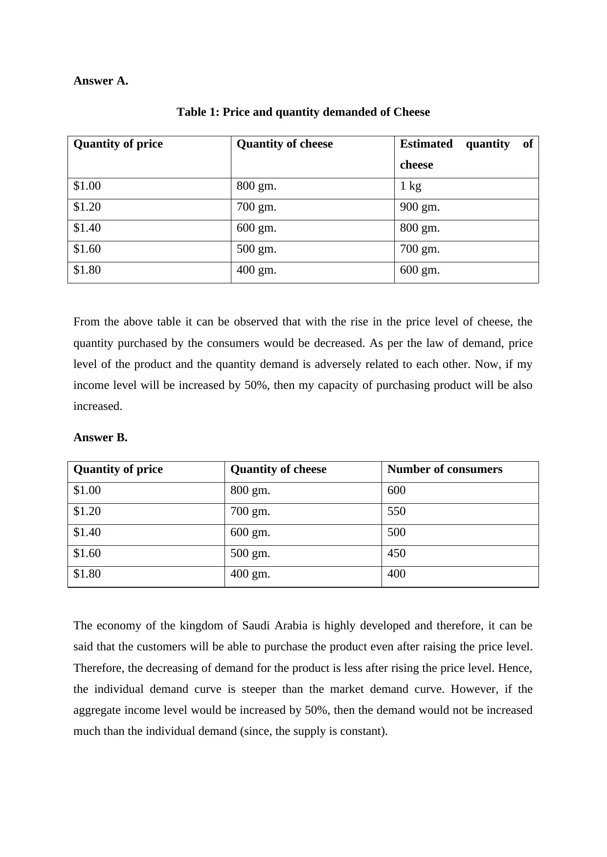
Answer A.
Table 1: Price and quantity demanded of Cheese
Quantity of price Quantity of cheese Estimated quantity of
cheese
$1.00 800 gm. 1 kg
$1.20 700 gm. 900 gm.
$1.40 600 gm. 800 gm.
$1.60 500 gm. 700 gm.
$1.80 400 gm. 600 gm.
From the above table it can be observed that with the rise in the price level of cheese, the
quantity purchased by the consumers would be decreased. As per the law of demand, price
level of the product and the quantity demand is adversely related to each other. Now, if my
income level will be increased by 50%, then my capacity of purchasing product will be also
increased.
Answer B.
Quantity of price Quantity of cheese Number of consumers
$1.00 800 gm. 600
$1.20 700 gm. 550
$1.40 600 gm. 500
$1.60 500 gm. 450
$1.80 400 gm. 400
The economy of the kingdom of Saudi Arabia is highly developed and therefore, it can be
said that the customers will be able to purchase the product even after raising the price level.
Therefore, the decreasing of demand for the product is less after rising the price level. Hence,
the individual demand curve is steeper than the market demand curve. However, if the
aggregate income level would be increased by 50%, then the demand would not be increased
much than the individual demand (since, the supply is constant).

Figure 1: Individual demand curve versus market demand curve
(Source: Green, Bean & Peterson, 2013)
DA and DB is individual demand curve, while DM is market demand curve.
Answer C.
Substitute good of cheese is butter and if the price level of substitute good will decrease by
50%, then the consumers will like to purchase it more over cheese.
Answer D.
Figure 2: Short run supply curve of cheese firm
(Source: Naumenko & Moosavian, 2016)
You're viewing a preview
Unlock full access by subscribing today!

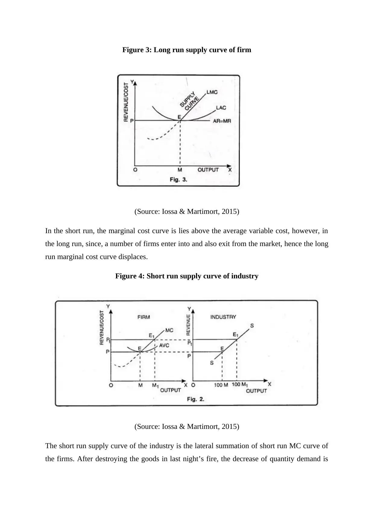
Figure 3: Long run supply curve of firm
(Source: Iossa & Martimort, 2015)
In the short run, the marginal cost curve is lies above the average variable cost, however, in
the long run, since, a number of firms enter into and also exit from the market, hence the long
run marginal cost curve displaces.
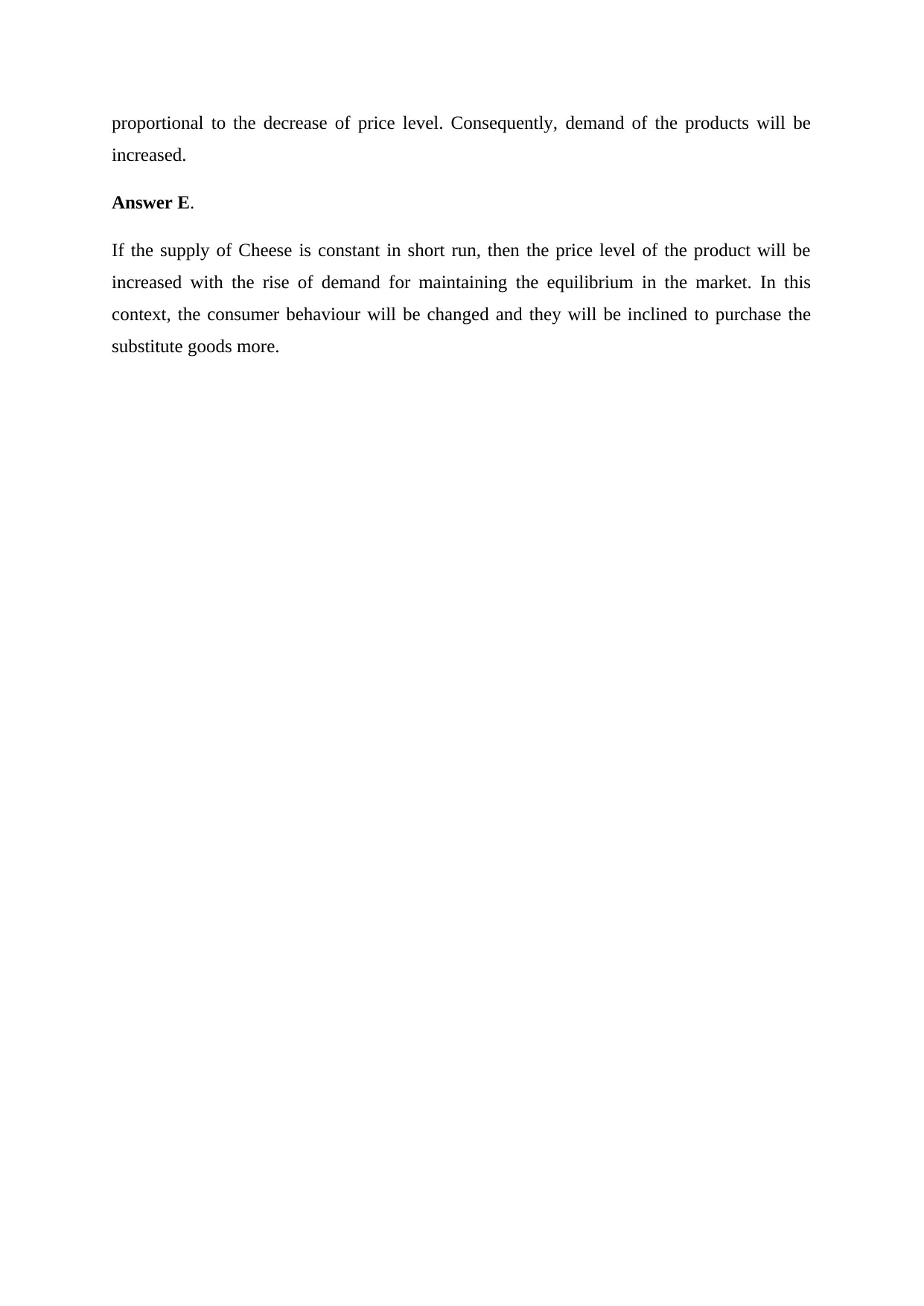
Figure 4: Short run supply curve of industry
(Source: Iossa & Martimort, 2015)
The short run supply curve of the industry is the lateral summation of short run MC curve of
the firms. After destroying the goods in last night’s fire, the decrease of quantity demand is
(Source: Iossa & Martimort, 2015)
In the short run, the marginal cost curve is lies above the average variable cost, however, in
the long run, since, a number of firms enter into and also exit from the market, hence the long
run marginal cost curve displaces.
Figure 4: Short run supply curve of industry
(Source: Iossa & Martimort, 2015)
The short run supply curve of the industry is the lateral summation of short run MC curve of
the firms. After destroying the goods in last night’s fire, the decrease of quantity demand is
Paraphrase This Document
Need a fresh take? Get an instant paraphrase of this document with our AI Paraphraser

proportional to the decrease of price level. Consequently, demand of the products will be
increased.
Answer E.
If the supply of Cheese is constant in short run, then the price level of the product will be
increased with the rise of demand for maintaining the equilibrium in the market. In this
context, the consumer behaviour will be changed and they will be inclined to purchase the
substitute goods more.

References
Green, G. P., Bean, J. C., & Peterson, D. J. (2013). Deep learning in intermediate
microeconomics: Using scaffolding assignments to teach theory and promote transfer. The
Journal of Economic Education, 44(2), 142-157.
Iossa, E., & Martimort, D. (2015). The simple microeconomics of public‐private partnerships.
Journal of Public Economic Theory, 17(1), 4-48.
Naumenko, A., & Moosavian, S. A. Z. N. (2016). Clarifying theoretical intricacies through
the use of conceptual visualization: Case of production theory in advanced microeconomics.
Applied Economics and Finance, 3(4), 103-122.
You're viewing a preview
Unlock full access by subscribing today!
1 out of 6
Related Documents

Your All-in-One AI-Powered Toolkit for Academic Success.
+13062052269
info@desklib.com
Available 24*7 on WhatsApp / Email
Unlock your academic potential
© 2024 | Zucol Services PVT LTD | All rights reserved.