Forecasting Methods for Airline Passenger Numbers using ARIMA Model and Regression

This study exhibits information about the variation in passenger numbers that will aid the management in adopting the necessary measures to curb the problem. Among the two methods, ARIMA is the best model in predicting the number of passengers. The study recommends the airline to have fully operational services before the peak season, whereby all the staffs should be available, thus reduce the running cost during the time.

1
Forecasting Methods
By:
Course Title:
Instructor:
Date:

2
Executive Summary
Various airlines have been declared bankrupt, such as the American (AAL), United
(UAL), and Delta (DAL) airlines; however, through merging with other airlines, they tend to
recover (Investopedia, 2019). Consequently, the closure of airlines tends to have multiple
adverse effects, which include loss of jobs, inconvenience to travellers, and losses to the
creditors (banks), among others. The following study seeks to exhibit information about the
variation in passenger numbers that will aid the management in adopting the necessary measures
to curb the problem. Among the two methods, ARIMA is the best model in predicting the
number of passengers. As evident, the magnitude of the seasonal fluctuations and the cyclic
movements do not change with the level of the time series; thus, the study used an additive
model. Besides, the highest seasonal factors are for July (63.831) whereas the lowest in
November (-53.9) thus indicating that was peak number of passengers in July and trough in the
number of passengers in November each year. Therefore, it is recommendable for the airline to
have fully operational services before the peak season, whereby all the staffs should be available,
thus reduce the running cost during the time.
Table of Contents

3
Executive Summary.............................................................................................................2
Introduction..........................................................................................................................4
Nature of Data......................................................................................................................5
Summary statistics...........................................................................................................5
Data in Action......................................................................................................................6
Predictive model..................................................................................................................9
Autoregressive Integrated Moving Average (ARIMA) Model.......................................9
Regression......................................................................................................................10
Conclusion and Recommendation.....................................................................................12
References..........................................................................................................................13
Appendix............................................................................................................................13

4
Introduction
There are no doubts the primary purpose of a business entity is to generate income, which
increases profits realized. However, in cases whereby the organization does not attain the above
objective, thus resulting in losses, it is essential to analyze the problem and adopt measures that
will not only curb the losses but also achieving stability. Notably, one of the industries that tend
to face numerous challenges, which tend to lead to losses is the airline industry. For instance,
various airlines have been declared bankrupt, such as the American (AAL), United (UAL), and
Delta (DAL) airlines; however, through merging with other airlines, they tend to recover
(Investopedia, 2019). Consequently, the closure of airlines tends to have multiple adverse effects,
which include loss of jobs, inconvenience to travellers, and losses to the creditors (banks),
among others.
Notably, there are numerous causes of losses in the airline industry, which include high
fixed and variable costs, exogenous events, reputation for hassles and poor services, among
others (Investopedia, 2019). The airlines need significant starting capital; as a result, they tend to
have substantial loan repayments regardless of the business conditions. Moreover, the industry
requires a large labor force to run complex operations, which increases the running cost. Besides,
fuel prices tend to face many price fluctuations, thus increasing operation costs, which may lead
to losses. Consequently, an area may face exogenous events, such as political instabilities,
terrorism, and natural disasters, which may increase the passenger demand. For instance, the US
airline industry experienced a loss of $7.7billion in 2001 due to a plunge in passenger demand
after the 9/11 attack. Generally, the fluctuations in the passenger demand may lead to losses;
thus, the airline needs to understand the levels of demand in various periods of the year.

5
As exhibited, the aviation industry (ABC) is facing a problem of fluctuating passenger
demand in the airport. As a result, it costs ABC several thousands of dollars to maintain the
airport services. Therefore, the following study seeks to exhibit information about the variation
in passenger numbers that will aid the management in adopting the necessary measures to curb
the problem.
Nature of Data
The data incorporates the number of passengers for 12 years (1949 to 1960) recorded in
each month.
Summary statistics
Min. 1st Qu. Median Mean 3rd Qu. Max.
104.0 180.0 265.5 280.3 360.5 622.0
As evident, the minimum number of passengers recorded was 104 whereas the maximum
number was 622. Besides, the mean and median number of passengers in each month were 280
and 365 respectively.
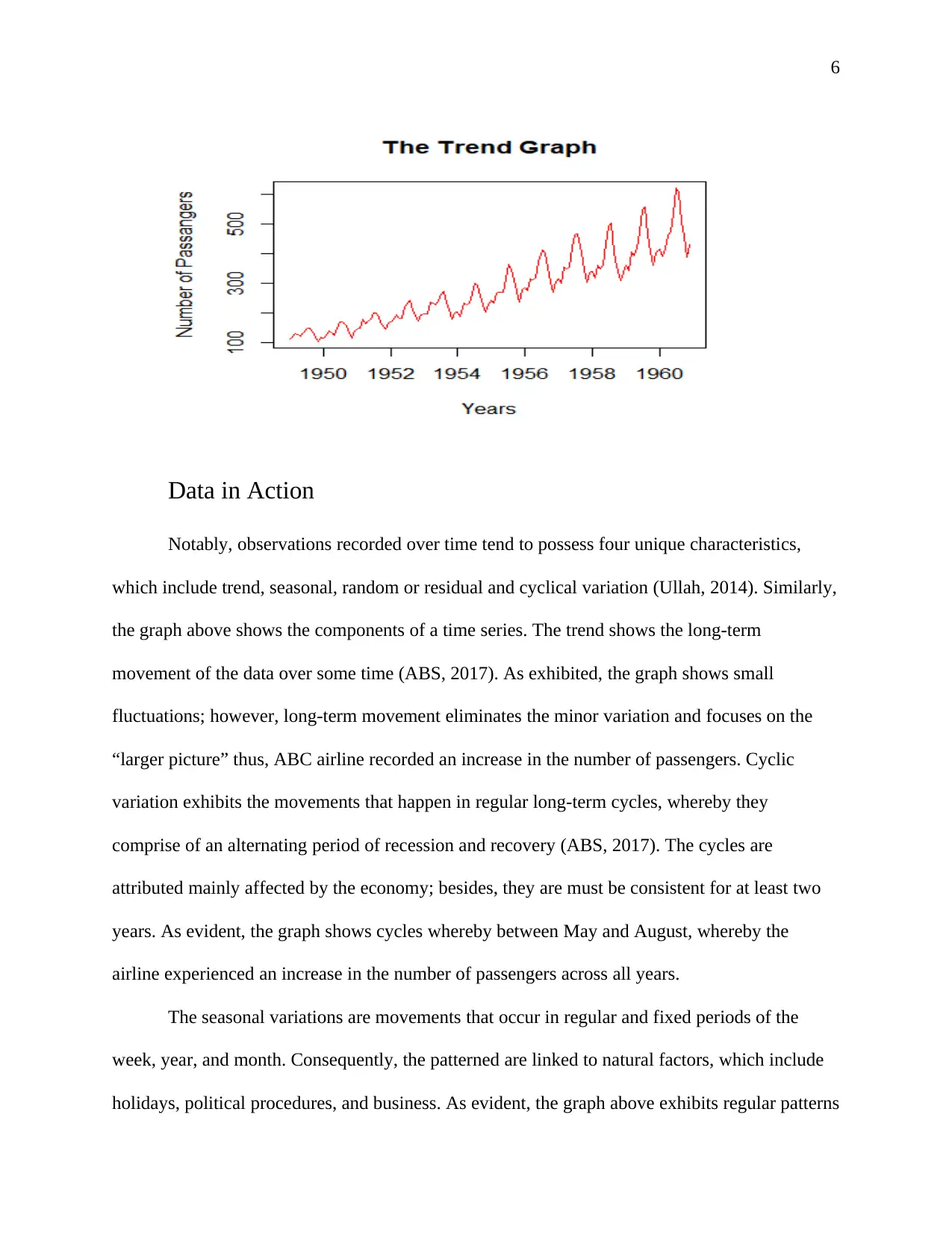
Consequently, it is essential to visualize the data to exhibit the trend to number of
passengers across the years. The graph below shows an increase in the number of passengers for
the 12 years.

6
Data in Action
Notably, observations recorded over time tend to possess four unique characteristics,
which include trend, seasonal, random or residual and cyclical variation (Ullah, 2014). Similarly,
the graph above shows the components of a time series. The trend shows the long-term
movement of the data over some time (ABS, 2017). As exhibited, the graph shows small
fluctuations; however, long-term movement eliminates the minor variation and focuses on the
“larger picture” thus, ABC airline recorded an increase in the number of passengers. Cyclic
variation exhibits the movements that happen in regular long-term cycles, whereby they
comprise of an alternating period of recession and recovery (ABS, 2017). The cycles are
attributed mainly affected by the economy; besides, they are must be consistent for at least two
years. As evident, the graph shows cycles whereby between May and August, whereby the
airline experienced an increase in the number of passengers across all years.
The seasonal variations are movements that occur in regular and fixed periods of the
week, year, and month. Consequently, the patterned are linked to natural factors, which include
holidays, political procedures, and business. As evident, the graph above exhibits regular patterns

7
across the 12 years. Notably, both the seasonal and cyclic variations are referred to as periodic
variations since they depend on a specific time. Notably, a time series data may exhibit
variations which are neither accounted for by seasonal nor cyclic variation. As a result, they are
accounted by the random variation since they tend to be unpredictable and are as a result of
chance events, such as exogenous events (war, fire, earthquakes, and terrorism, among others).
Although it is minimal, the graph above exhibits residual.
Therefore, to develop an efficient and accurate forecast, it is essential to quantify the
above components by decomposing the data. There are two methods used to decompose the data,
which include the multiplicative and additive model (Hyndman, 2019). The additive model is
applicable when the magnitude of the seasonal fluctuations or when the cyclic movements do not
change with the level of the time series. On the other hand, the multiplicative model is used
when both the seasonal and cyclic variations appear proportional to the level of the time series.
Additive model = T + S + C + R
Whereby T = trend
S = Seasonal variation
C = Cyclic variation
R = Random variation
Notably, S, C, and R are expressed as absolute values.
Multiplicative model = T * S * C * R
Whereby S, C, and R are expressed as proportion or percentage.
Since, the magnitude of the seasonal fluctuations or when the cyclic movements do not
change with the level of the time series then the study will use an additive model.

8
For instance, the table below show the seasonal factors for each month (January to
December), which are equal across the years.
Jan Feb March April May June July Aug Sept Oct Nov Dec
24.749 -36.19 -2.241 -8.037 -4.506 25.403 63.831 62.823 16.52 -20.64 -53.9 -28.61
The highest seasonal factors are for July (63.831) whereas the lowest is November (-
53.9) thus indicating that was peak number of passengers in July and trough in number of
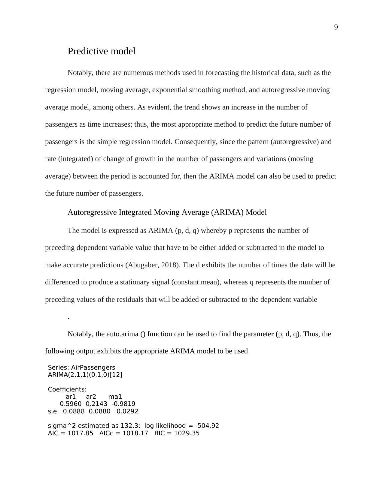
passengers in November each year. The following graph exhibits the estimated trend, seasonal,
random components of the data.

9
Predictive model
Notably, there are numerous methods used in forecasting the historical data, such as the
regression model, moving average, exponential smoothing method, and autoregressive moving
average model, among others. As evident, the trend shows an increase in the number of
passengers as time increases; thus, the most appropriate method to predict the future number of
passengers is the simple regression model. Consequently, since the pattern (autoregressive) and
rate (integrated) of change of growth in the number of passengers and variations (moving
average) between the period is accounted for, then the ARIMA model can also be used to predict
the future number of passengers.
Autoregressive Integrated Moving Average (ARIMA) Model
The model is expressed as ARIMA (p, d, q) whereby p represents the number of
preceding dependent variable value that have to be either added or subtracted in the model to
make accurate predictions (Abugaber, 2018). The d exhibits the number of times the data will be
differenced to produce a stationary signal (constant mean), whereas q represents the number of
preceding values of the residuals that will be added or subtracted to the dependent variable
.
Notably, the auto.arima () function can be used to find the parameter (p, d, q). Thus, the
following output exhibits the appropriate ARIMA model to be used
Series: AirPassengers
ARIMA(2,1,1)(0,1,0)[12]
Coefficients:
ar1 ar2 ma1
0.5960 0.2143 -0.9819
s.e. 0.0888 0.0880 0.0292
sigma^2 estimated as 132.3: log likelihood = -504.92
AIC = 1017.85 AICc = 1018.17 BIC = 1029.35

10
Therefore, the best model is ARIMA(2, 1, 1)(0,1,0)
The following table exhibits the prediction of the number of passengers using the above
model for the next one year (1961)
Point Forecast Lo 99.5 Hi 99.5
Jan 1961 475.5508 401.2319 549.8698
Feb 1961 460.3651 386.7197 534.0106
Mar 1961 462.5868 386.8532 538.3203
Apr 1961 508.3603 423.2026 593.5180
May 1961 514.0491 425.9615 602.1368
Jun 1961 535.6131 441.7452 629.4810
Jul 1961 593.8589 487.4450 700.2728
Aug 1961 580.1304 473.8675 686.3933
Sep 1961 524.9834 426.7108 623.2560
Oct 1961 511.7557 413.8814 609.6300
Nov 1961 474.2690 381.6207 566.9173
Dec 1961 494.2778 395.6777 592.8779
Regression
As exhibited the graph exhibited and upward linear trend thus regression model can be
used to estimate the future number of passengers expected to use the airline. The method of least
square can be used to find the best fit line relationship (line of best fit) between two variables.
The equation of a straight line used to describe the linear relationship between the independent
variables X and the dependent variable Y;
Y = B + B1X
Whereby B is the intercept of the Y axis and B1 is the gradient or the slope of the straight
line.
In a time-series analysis, the independent variable is time, so t can be interchanged with
X and Yt be switched with Y hence the equation becomes;
Yt = B + B1t
Whereby Yt is the forecast value of the time series in period t

11
Therefore, the following output exhibits the coefficients of an autoregressive model
(linear regression)
ar(x = SeasonalAdj_AirPassengers, aic = T)
Coefficients:
1 2 3 4 5 6 7 8 9 10 11 12 13
0.9325 0.1655 -0.1196 0.0514 0.0566 -0.1963 -0.0008 -0.0088 -0.0455 0.0857
0.2458 0.0880 -0.2836
Order selected 13 sigma^2 estimated as 602
The following table exhibits the prediction of the number of passengers using the above
model for the next one year (1961)
1961 Sep Prediction
Jan 431.0250 24.53641
Feb 408.7673 33.54893
Mar 403.1615 42.07658
Apr 405.6619 48.70613
May 415.5786 55.02599
Jun 435.2423 61.49864
Jul 450.4400 66.27188
Aug 440.9775 70.05146
Sep 427.5926 72.70307
Oct 420.2575 74.36941
Nov 414.4302 75.62476
Dec 409.2294 77.47639
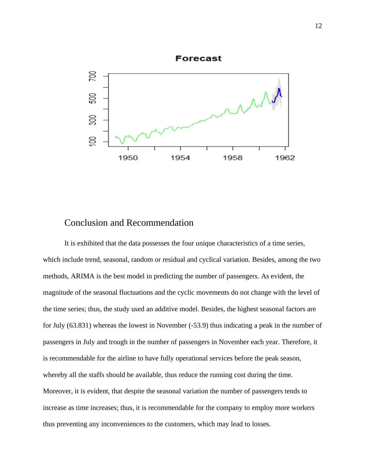
The graph below shows the prediction (blue) of the number of passengers using the
ARIMA model, which tends to conform with the data, thus ARIMA is the most appropriate
model to predict the expected number of passengers in the future. Notably, the prediction is for
the seasonally adjusted data of the number of passengers

12
Conclusion and Recommendation
It is exhibited that the data possesses the four unique characteristics of a time series,
which include trend, seasonal, random or residual and cyclical variation. Besides, among the two
methods, ARIMA is the best model in predicting the number of passengers. As evident, the
magnitude of the seasonal fluctuations and the cyclic movements do not change with the level of
the time series; thus, the study used an additive model. Besides, the highest seasonal factors are
for July (63.831) whereas the lowest in November (-53.9) thus indicating a peak in the number of
passengers in July and trough in the number of passengers in November each year. Therefore, it
is recommendable for the airline to have fully operational services before the peak season,
whereby all the staffs should be available, thus reduce the running cost during the time.
Moreover, it is evident, that despite the seasonal variation the number of passengers tends to
increase as time increases; thus, it is recommendable for the company to employ more workers
thus preventing any inconveniences to the customers, which may lead to losses.

13
References
ABS. (2017, March 27). Time Series. Retrieved from Australian Bureau of Statitistics Website:
https://www.abs.gov.au/websitedbs/d3310114.nsf/home/time+series+analysis:+the+basics
Abugaber, D. (2018). A Language, not a Letter: Learning Statistics in R: Using ARIMA for Time
Series Analysis. Retrieved from https://ademos.people.uic.edu/Chapter23.html
Hyndman, R. (2019, March 4). Time Series Decomposition. Retrieved from
http://course1.winona.edu/bdeppa/FIN%20335/Handouts/Time_Series_Decomposition.html
Investopedia. (2019, June 25). 4 Reasons Why Airlines Are Always Struggling . Retrieved from
Ivestopedia Website: https://www.investopedia.com/financial-edge/0510/4-reasons-why-airlines-
are-always-struggling.aspx
Ullah, M. I. (2014, June 15). Component of Time Series Data . Retrieved from Basic Statistics
and Data Analysis Website:
https://itfeature.com/time-series-analysis-and-forecasting/component-of-time-series-data
Appendix
# Loading the data
data(AirPassengers)
# Viewing of the data
AirPassengers
# The summary or descriptive statistics
summary (AirPassengers)
# The trend graph
plot(AirPassengers, xlab ="Years", ylab ="Number of Passangers", main = "The Trend Graph",
col ="red")
# Decomposing
AirPassengegers_Decomposition<- decompose(AirPassengers)
#The estimated trend, seasonal, random components of the data.
plot(AirPassengegers_Decomposition, xlab ="Years", col ="Blue")
#Seasonally Adjusted Airpassenger data
SeasonalAdj_AirPassengers<-seasadj(AirPassengegers_Decomposition)
#ARIMA model

14
#Finding the parameters(p, d, q)
auto.arima (AirPassengers)
#ARIMA Prediction
ARIMA_PREDICTION<-forecast(SeasonalAdj_AirPassengers, h=12, level=c(99.5))
#Regression Prediction
REGRESSION_PREDICTION<-ar(SeasonalAdj_AirPassengers, aic = T)