Financial Derivatives: Pricing ZCB, Forwards, Futures, Options
VerifiedAdded on 2023/01/20
|6
|1097
|27
Homework Assignment
AI Summary
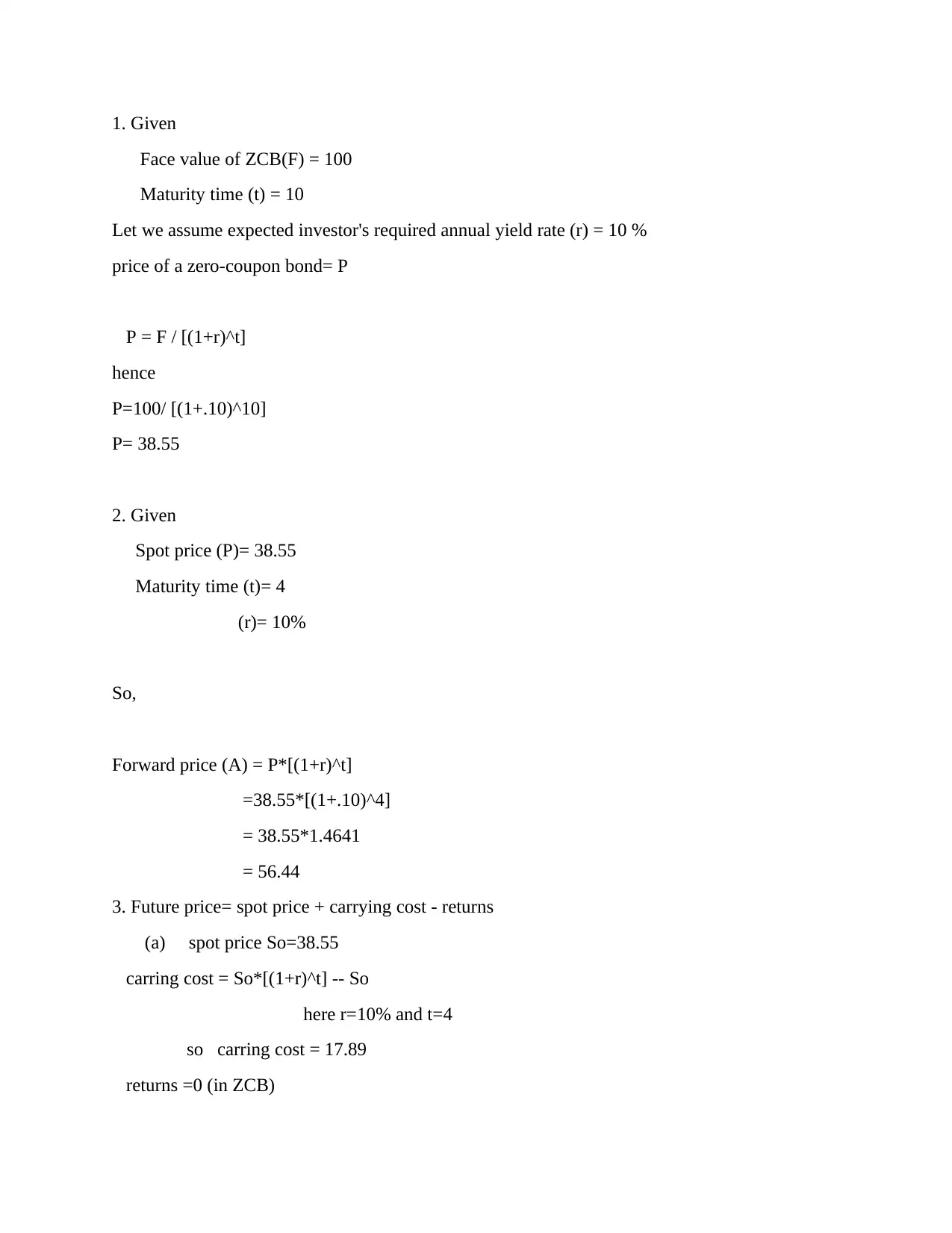
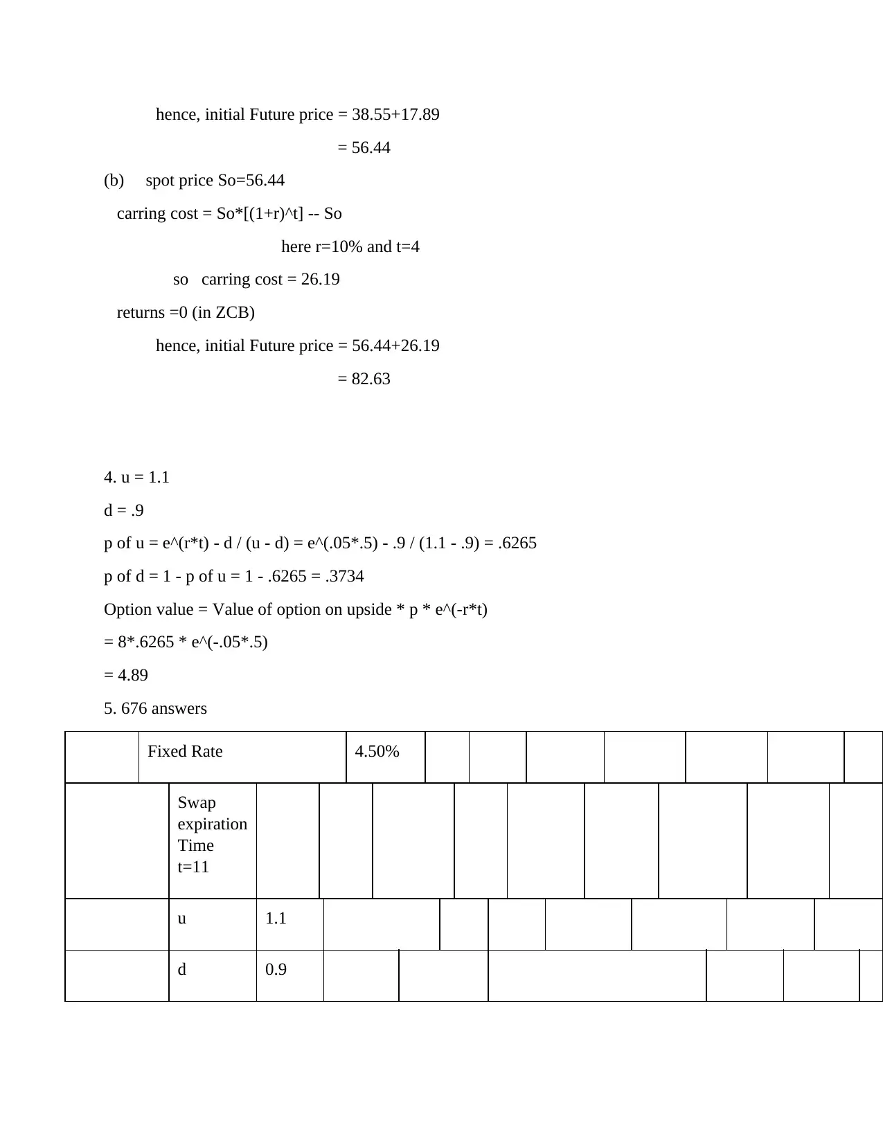
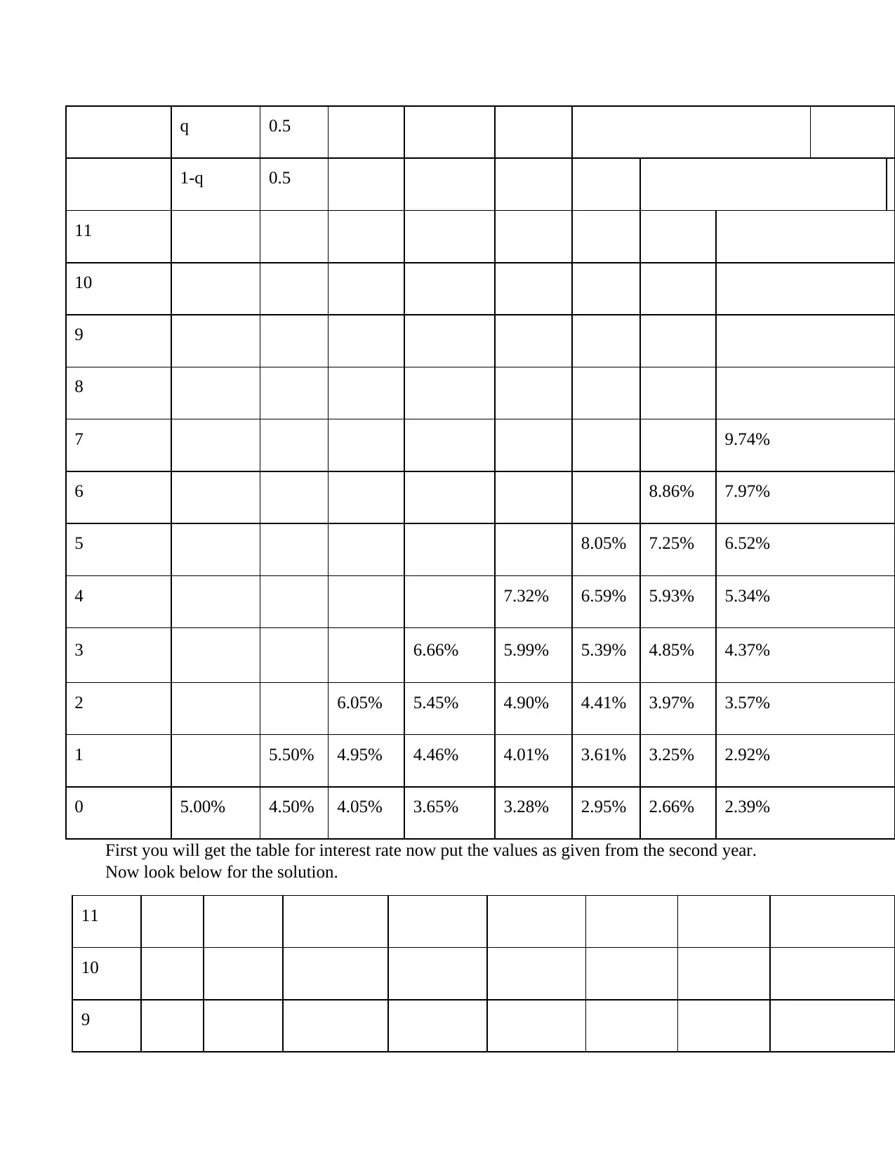
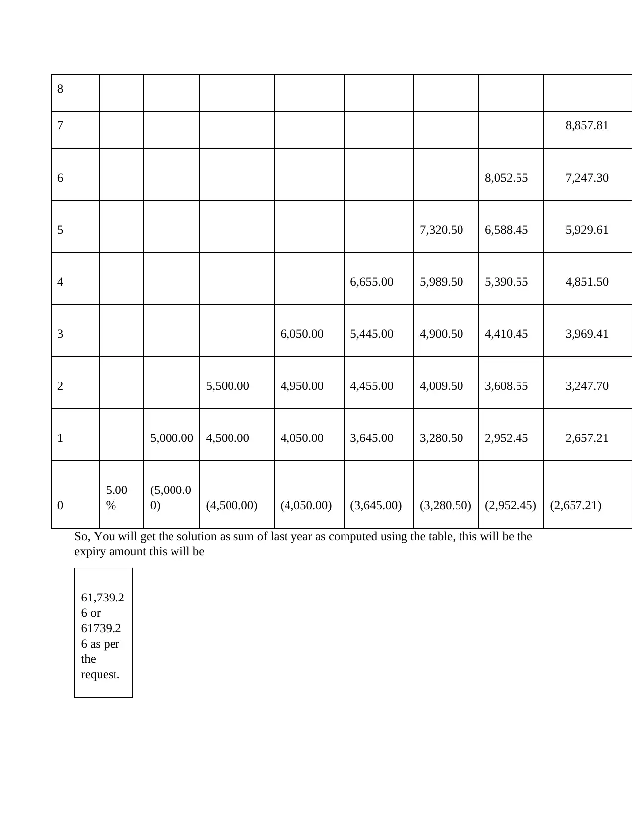
This document presents a comprehensive solution to a finance assignment focused on the valuation and pricing of various financial derivatives. The solution begins with the calculation of the price of a zero-coupon bond (ZCB) based on its face value, maturity time, and expected yield rate. It then proceeds to determine the forward price of an asset, considering spot price, maturity time, and interest rates. The assignment also explores the calculation of future prices, taking into account spot prices, carrying costs, and returns. Furthermore, the solution includes the valuation of options using the binomial option pricing model, demonstrating the calculation of option values based on up and down movements, probabilities, and risk-free rates. Finally, the assignment addresses the pricing of a fixed-rate swap using a binomial tree, providing a step-by-step approach to determine the swap's value and expiry amount. The solution incorporates the use of relevant formulas and calculations, providing a detailed and practical understanding of financial derivatives pricing.
1 out of 6


Your All-in-One AI-Powered Toolkit for Academic Success.
+13062052269
info@desklib.com
Available 24*7 on WhatsApp / Email
![[object Object]](/_next/static/media/star-bottom.7253800d.svg)
Copyright © 2020–2026 A2Z Services. All Rights Reserved. Developed and managed by ZUCOL.