Identifying Relevant Time Series for Forecasting Danish Tourists to Australia

This document discusses the process of identifying a relevant time series for forecasting Danish tourists to Australia. It explores the systematic components of the time series, including trend, seasonality, cyclical variation, and irregular movement. The document also examines the economic and environmental factors influencing the time series and suggests appropriate methods for smoothing the data. Additionally, it provides insights into evaluating and selecting the optimal model for forecasting the time series.

1. “Identify a relevant time series for the visitors arriving to Australia from your airline’s
home country (for at least the last 20 years) which may be useful in generating the
forecasts required by your airline. You may merge time series if you deem this is
necessary. Justify your choice/s.”
“Data should be available through the Australian Bureau of Statistics (ABS).”
“Provide a line chart of the relevant time series for approximately the last 20 years.”
2. “Comment in general on the characteristics of the time series line chart. What
systematic components are evident in the time series? Explain your answer.”
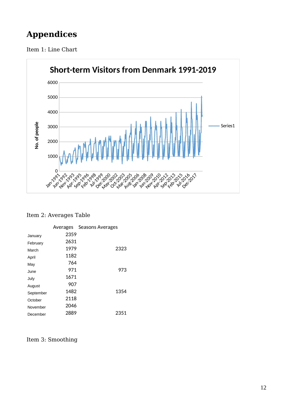
The data used was the short-term visitors to Australia data collected with regard to
country of residency; columns related to data from other countries were removed.
Data represented in the line chart in the appendix is for the past 27 years between
January 1991 and February 2019. With regard to the four components of time series
data we can check the trend, seasonal movement, cyclical movement, and irregular
movement.
Trend
The trend documents the long term movement of Denmark visitors to Australia. The
trend has an upwards movement between 1991 and 2019 indicating that the number
of short-term Denmark visitors to Australia has been increasing over the years
between the specified period. The peaks clearly indicated that in the long run the
highest number of annual Danish tourists has increased significantly. The troughs on
the other hand indicate that the long run lowest number of annual Danish tourist has
not change significantly over the year; especially between 2000 and 2019.
Seasonality
Seasonal movement indicates that the movement of Demark visitor change depending
on the time of the year there are months like January and December when the
numbers are considerably high. In other months like August and July the number of
Denmark visitors is considerably low. There is a difference between the numbers of
Danish tourists visiting Australia at different times of the years. It seems like the
highest numbers of Danish tourists are recorded during the first and fourth quarters
of the year. As a result, few Danish tourist tour Australia during the second and third
quarters of any given year.
Cyclical Variation
Cyclical variation is not critically evident because the influx of Denmark visitors does
not seem to be affected by financial and economic changes e.g. the great recession of
2000s. However, we can see that the troughs of the line seems to level out during the
2000s this could be an indication that to a small degree the number of Danish people
visiting Australia is affected by financial crisis and market instabilities in Europe.
Irregular Movement
Lastly, looking at the data we cannot see any irregular movements in data for the
period between 1991 and 2019. There is only a slight irregular movement in the
overall upwards movement of the chart documented between 2001 and 2005: this
period realized a plateau in the number of Denmark visitors touring Australia. This
1

can be attributed to a number of unexpected events such as an increased desire by
Danish people to explore other parts of the worlds like Africa.
(Appendix Item 1)
2

3. “Confirm the presence of the systematic components of the time series using relevant
tools and measures. Explain your answer.”
4. “Outline the economic and environmental factors or circumstances which are likely to
have influenced the characteristics or components of the time series. Will these
factors or circumstances apply to the relevant forecasting period? Explain your
answer.”
Looking at the monthly and seasonal averages for all 26 years we see that Denmark
tourists normally visit Australia in high number during the 1st and 4th quarters of the
year (average table in appendix). The averages were calculated by arranging the data
in terms of months and then computing the averages for all months across all years.
We can see from the results above that the numbers for each season are different
indicating that the data does demonstrate seasonality. An ANOVA test to assess the
difference between means for the seasons was performed to determine whether the
assumption of seasonality was valid. The ANOVA results indicated in Table 1
demonstrate that seasonality is statistically significant because we will reject the null
hypothesis that the means are equivalent for all quarters 0f the year (Hartshorn,
2017).
The seasonality is caused by favorable climatic conditions induced by the summer
season. More tourists will seek to travel to destinations with warm weather compared
to those who are willing to visit the same locations during less favorable times of the
year. The economic factor influencing this seasonal change in Demark tourist influx is
due to a difference in income levels. Well off individuals and families will seek to
vacation during the most suitable weather conditions regardless of the costs.
However, less well off individuals and families will go on trips when the costs are not
so high. The number of people who will pay for the summer season will be higher than
that of people going to Australia from Denmark during other seasons. There is a
smooth transition in the number of Danish people visiting Australia during the high
and low season. For example, April marks the end of the first period of high influx of
tourist and indicates the starts of the low season of Danish travelers. April has an
average figure of visitors that indicates a smooth transition from the low to the high
season; A similar observation can be made for September. Both high seasons have
annual averages in Danish tourist visits that are almost similar; while, the averages
recorded in the individual low seasons are considerably different. The difference in
the low seasons is an indication that Danish visitors are more prone t visiting Australia
in the third quarter of the year before the onset of the high season in the fourth
quarter.
3

The forecasts made also have take into account the systematic movement in Danish
tourists’ visits for them to be realistic. As such, a good forecast model should be able
to showcase the difference in tourist influx from one quarter to the next without
altering the perception of high and low seasons.
(Appendix Item 2)
4

5. “Without applying a decomposition, apply an appropriate method in EXCEL to smooth
(remove randomness) the chosen time series for the last 4 years to help further
identify the relevant systematic components. Explain what you have done.”
The data for the last four years was copied from January 2015 to February 2019 and
pasted in another worksheet. A column for the period was added between the data and
the tourist visits for the past four years. The data was smoothened using exponential
smoothing. The process involve going to the Data tab, clicking on data analysis and
selecting exponential smoothing. In the exponential smoothing dialog box we will
input the range for tourist visits for the past four years. We will us a dumping factor
of 0.75 that will not extremely smoothen out the data but will eliminate randomness.
The output range was selected as the column adjacent to the one containing the
Denmark tourist inflow history for the past four years.
Looking at the output the influx data of Danish tourist seems to be considerably more
ironed out without any random spikes in the number of travelers observed in a given
monthly. As such, the 0utput data was significantly different from the original data for
the same four year period. The exponential smoothing curve generated for the new
data demonstrates seasonality more clearly compared to a line chart drawn for the
original data for the same period. The curve for the new data is smooth and void of
sharp dips and spikes that are caused by randomness. Through the removal of
randomness one can clearly see the seasonal nature of data indicating the Danish
travelers are prone to visiting Australia at the begin and end of any given year. Fewer
Danish people are willing to explore Australia at the middle of the year.
(Appendix Item 3)
5

6. “From the results of the above smoothing, provide a time series line chart comparing
the original time series with the generated smoothed values. Comment on your
smoothing.”
“Include the forecasts from #10 as part of your line chart above.”
In this segment we are trying to eliminate randomness from the time series data as a
way of increasing the visibility of seasonality in the data. Randomness refers to the
present of data point that seems to follow no particular pattern and therefore appear
randomly on the line chart distorting the overall trend in the data. By removing
randomness we should be able to get a definitive feel over the data pattern. A smooth
curve is also expected hat is devoid of sharp turns or corners there should be fluid
movement from peak to trough and from trough to peak .
The line output of the smoothing process is different from the original data line
indicating that randomness has been eliminated because the movement of the data is
considerably much smoother than that of the original data over the 4 years period.
The seasonal pattern in the data is considerably much clearer in the new curve for
smoothened forecasts allowing us to understand the influx of Danish people in
Australia at different times of the year. The exponential smoothing was not so
extreme as to eliminate seasonality but it was sufficient to eradicate a considerable
amount of randomness. It is clear that the amplitude (distance between the peaks and
troughs) for the new smoothened data is considerably short compare to that observed
in the original data. The smoothing process eliminates extremes in the peaks and
troughs to ensure that the data transitions smoothly from one month to the next. As a
result, the figures of Danish tourists visiting Australia under the new data are not as
high or low as in the original data.
(Appendix Item 4)
6

7. “Perform the appropriate tests for whether your model has captured all the systematic
components and/or whether the errors are random. Explain your answer.”
8. “Do the results in #6 and #7 suggest any re-evaluation or modification, if at all?
Explain your answer.”
In model selection the first model may not be the optimal model. Therefore, there is
need to assess several other model options with variations being made to given
parameters. Here the parameter that will be adjusted in the pursuit of the
optimal/best model is the dumping factor used in the exponential smoothing process.
The smoothing technique employed is exponential smoothing it relies of the usage of a
dumping factor to determine to what degree smoothing is carried out. The dumping
factor is a value between 0 and 1. The data becomes more smoothed out as the
dumping factor tends towards 1 and the data becomes less smoothed out as the
dumping factor approaches zero.
The best test to assess whether the optimal model was selected is through the
computation of MSE (Mean Squared Error) for different models generated with
varying dumping factors. Nevertheless, the smoothing on the data still has to remain
regardless of assessing which model has the smallest MSE. Four comparison m0dels
were drawn are different dumping factors. The first model was using a dumping factor
of 0.9 the model was sensitive to seasonality however the forecasted values were
considerably different from the actual data; meaning the amplitudes for the peaks and
troughs were too narrow. The same conclusion was reached with regard to the model
generated using dumping factor of 0.8. The models generate using a dumping factor of
less than 0.7 were unable to effectively eliminate randomness from the original data;
as a result, the models are unable to paint a clear picture of seasonality. This sort of
inadequacy was the case with regard to the two models generated with dumping
factors of 0.5 and 0.6. From the assess we see that the model we selected with a
dumping factor of 0.75 is optimal regardless of its large MSE. Therefore, based on the
computations made in Question 6 and 7 there will be no need for modification or re-
evaluation because the original model with a factor of 0.75 was the best
(Appendix Item 5)
7

9. “Using the results of the smoothing method you applied, provide numerical estimates
for the underlying systematic components (for example, if a trend is observed provide
a relevant trend equation and/or if seasonality is observed provide estimates of the
seasonal relatives or indexes).”
“Using your results, provide an appropriate time series model for the time series you
selected in #1.”
“Critically evaluate your choice of model.”
January February March April May June July August September October November December
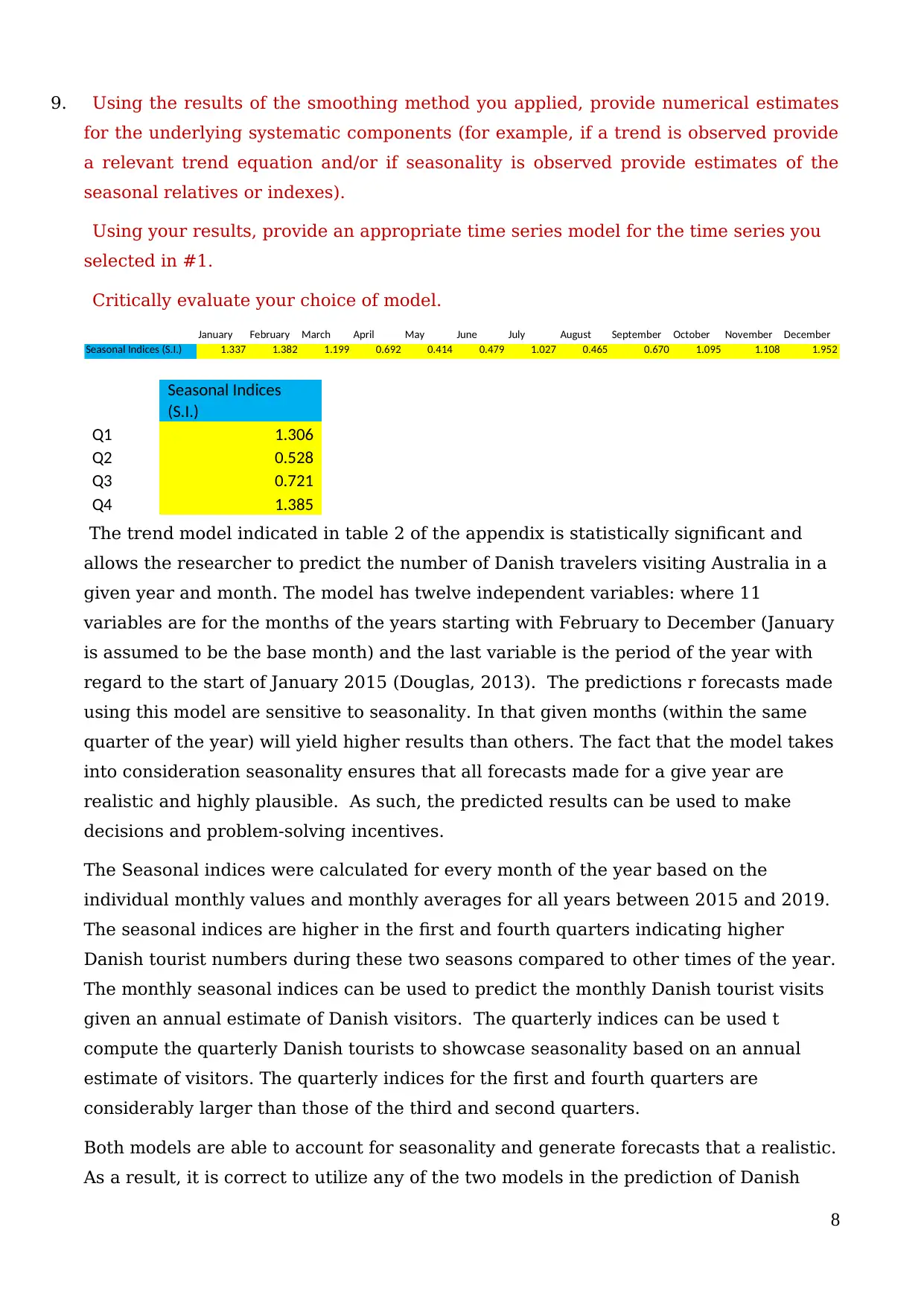
Seasonal Indices (S.I.) 1.337 1.382 1.199 0.692 0.414 0.479 1.027 0.465 0.670 1.095 1.108 1.952
Seasonal Indices
(S.I.)
Q1 1.306
Q2 0.528
Q3 0.721
Q4 1.385
The trend model indicated in table 2 of the appendix is statistically significant and
allows the researcher to predict the number of Danish travelers visiting Australia in a
given year and month. The model has twelve independent variables: where 11
variables are for the months of the years starting with February to December (January
is assumed to be the base month) and the last variable is the period of the year with
regard to the start of January 2015 (Douglas, 2013). The predictions r forecasts made
using this model are sensitive to seasonality. In that given months (within the same
quarter of the year) will yield higher results than others. The fact that the model takes
into consideration seasonality ensures that all forecasts made for a give year are
realistic and highly plausible. As such, the predicted results can be used to make
decisions and problem-solving incentives.
The Seasonal indices were calculated for every month of the year based on the
individual monthly values and monthly averages for all years between 2015 and 2019.
The seasonal indices are higher in the first and fourth quarters indicating higher
Danish tourist numbers during these two seasons compared to other times of the year.
The monthly seasonal indices can be used to predict the monthly Danish tourist visits
given an annual estimate of Danish visitors. The quarterly indices can be used t
compute the quarterly Danish tourists to showcase seasonality based on an annual
estimate of visitors. The quarterly indices for the first and fourth quarters are
considerably larger than those of the third and second quarters.
Both models are able to account for seasonality and generate forecasts that a realistic.
As a result, it is correct to utilize any of the two models in the prediction of Danish
8

tourist short-term visits to Australia. However, it is unlikely that both models will
develop the same values for the same month of a given year. Nevertheless, we should
not expect there to be considerable difference in the values generate under each
model.
(Appendix Item 6 and Item 7)
9

10. “Use EXCEL to provide relevant monthly forecasts for total visitor arrivals from your
airline’s home country to Australia for each month beyond the sample data period (one
year of monthly out-of-sample forecasts). Compare and contrast your forecasts using
MINITAB. Comment on any differences you observe between the two sets of
forecasts.”
“Explain why (or why not) such a time frame (one year of monthly out-of-sample
forecasts) beyond the sample period would be appropriate for the launch of new air
travel routes.”
“Critically evaluate the factors you would need to consider when forecasting for the
second or third year (of monthly forecasts) beyond the sample period.”
The forecast in table 3 and table 4 are generated using seasonal indices and trend
model respectively. The overall average for the past four years 2015 to 2018 was used
as the average for the entire year of 2019. The average was multiplied with the
respective seasonal index for each month in the year. The trend model was computed
using the values of 12 variables for all months of 2019. The two sets of forecasts were
compared in Minitab to assess the similarities and differences in the monthly
forecasts.
Looking at the results for the two sample t-test in Minitab we see that we will not
reject the null hypothesis (Gaston, 2014). As such, we will conclude that the difference
between the two samples is not statistically significant. The forecasts for both was
sensitive to seasonal changes indicating higher figures of Danish tourists during the
first and last three months of the years compared to the middle six months of the
years. However, the number of tourists forecasted in each month was higher in the
results generated using the trend model compared to those generated using the
seasonal indices. The reason why the forecasts were conducted for an entire year was
to identify whether the forests generated were sensitive to seasonality in the time
series data. From chart 1 and 2 in the appendix we can see that both forecasts are
sensitive to seasonality and they follow the same path i.e. pattern regardless of
forecasting technique used.
The factors that would need to be considered when forecasting 2 or 3 years beyond
the stipulated sample period are seasonality and trend; contrary to forecasting for 1
year beyond the sample period where we would only use the seasonality factor. These
two factors ensure that any data generated does not only adhere to the seasonality
pattern but also follows the long-turn growth pattern in the Number of Danish tourists
who visit Australia.
(Appendix Item 8 to Item 12)
10

References
Douglas, C. M. (2013). Introduction to Linear Regression Analysis (5th Edition ed.).
Hoboken, New Jersey: John Wiley & Sons.
Gaston, L. (2014). Hypothesis Testing Made Simple (1st Edition ed.). Leonard Gaston .
Hartshorn, S. (2017). Hypothesis Testing: A Visual Introduction to Statistical
Significance (1st Edition ed.). San francisco, CA : Independently Published.
11

Appendices
Item 1: Line Chart
Jan-1991
Jun-1992
Nov-1993
Apr-1995
Sep-1996
Feb-1998
Jul-1999
Dec-2000
May-2002
Oct-2003
Mar-2005
Aug-2006
Jan-2008
Jun-2009
Nov-2010
Apr-2012
Sep-2013
Feb-2015
Jul-2016
Dec-2017
0
1000
2000
3000
4000
5000
6000
Short-term Visitors from Denmark 1991-2019
Series1
No. of people
Item 2: Averages Table
Averages Seasons Averages
January 2359
February 2631
March 1979 2323
April 1182
May 764
June 971 973
July 1671
August 907
September 1482 1354
October 2118
November 2046
December 2889 2351
Item 3: Smoothing
12

1
4
7
10
13
16
19
22
25
28
31
34
37
40
43
46
49
0
500
1000
1500
2000
2500
3000
3500
Exponential Smoothing
Forecast
Data Point
Value
Item 4: Smoothened Vs Original
1
4
7
10
13
16
19
22
25
28
31
34
37
40
43
46
49
0
1000
2000
3000
4000
5000
6000
Comparison of Original and Smoothened
Tourist Numbers
Forecast
N0. of Tourists
Item 5: Best Smoothened Model
1
4
7
10
13
16
19
22
25
28
31
34
37
40
43
46
49
0
500
1000
1500
2000
2500
3000
3500
4000
Best Model
factor 0.6
factor 0.5
factor 0.9
factor 0.8
No of People
13

Item 6: Tables 1
Anova: Single Factor
SUMMARY
Groups Count Sum Average Variance
Season 1 3 6968.227 2322.742 107392.4588
Season 2 3 2917.857 972.619 43652.21088
Season 3 3 4060.714 1353.571 158431.1224
Season 4 3 7053.571 2351.19 218435.3741
ANOVA
Source of Variation SS df MS F P-value F crit
Between Groups 4352821.111 3 1450940 10.99382217 0.003282 4.066181
Within Groups 1055822.333 8 131977.8
Total 5408643.443 11
Item 7: Tables 2
SUMMARY OUTPUT
Regression Statistics
Multiple R 0.989725
R Square 0.979557
Adjusted R Square 0.972926
Standard Error 183.7748
Observations 50
ANOVA
df SS MS F Significance F
Regression 12 59875393 4989616 147.7391 1.91E-27
Residual 37 1249607 33773.17
Total 49 61125000
CoefficientsStandard Error t Stat P-value Lower 95% Upper 95%Lower 95.0%Upper 95.0%
Intercept 3135.774 94.06755 33.33534 3.33E-29 2945.175 3326.373 2945.175 3326.373
Period 11.36905 1.830441 6.211099 3.25E-07 7.660223 15.07787 7.660223 15.07787
M2 108.631 116.2438 0.93451 0.3561 -126.901 344.1632 -126.901 344.1632
M3 -549.524 123.4971 -4.44969 7.61E-05 -799.753 -299.295 -799.753 -299.295
M4 -1760.89 123.4021 -14.2696 1.28E-16 -2010.93 -1510.86 -2010.93 -1510.86
M5 -2422.26 123.3342 -19.6398 3.66E-21 -2672.16 -2172.36 -2672.16 -2172.36
M6 -2283.63 123.2935 -18.5219 2.63E-20 -2533.45 -2033.81 -2533.45 -2033.81
M7 -995 123.2799 -8.07107 1.12E-09 -1244.79 -745.211 -1244.79 -745.211
M8 -2331.37 123.2935 -18.9091 1.31E-20 -2581.19 -2081.55 -2581.19 -2081.55
M9 -1867.74 123.3342 -15.1437 1.94E-17 -2117.64 -1617.84 -2117.64 -1617.84
M10 -879.107 123.4021 -7.12392 1.94E-08 -1129.14 -629.071 -1129.14 -629.071
M11 -865.476 123.4971 -7.00807 2.77E-08 -1115.71 -615.247 -1115.71 -615.247
M12 1123.155 123.6191 9.085607 5.86E-11 872.6786 1373.631 872.6786 1373.631
14

Item 8: Table 3
Average for 2019 2354
Seasonal Indices (S.I.) Forecast 2019
January 1.337 3148
February 1.382 3254
March 1.199 2822
April 0.692 1628
May 0.414 976
June 0.479 1127
July 1.027 2417
August 0.465 1095
September 0.670 1577
October 1.095 2578
November 1.108 2608
December 1.952 4596
Item 9: Table 4
Forecast for 2019 Period
1 3693 49
2 3813 50
3 3166 51
4 1966 52
5 1316 53
6 1466 54
7 2766 55
8 1441 56
9 1916 57
10 2916 58
11 2941 59
12 4941 60
Item 10: Table 5
Two-Sample T-Test and CI: Forecast S.I., Forecast Trend Model
Two-sample T for Forecast S.I. vs Forecast Trend Model
N Mean StDev SE Mean
15

Forecast S.I. 12 2319 1083 313
Forecast Trend Model 12 2695 1118 323
Difference = μ (Forecast S.I.) - μ (Forecast Trend Model)
Estimate for difference: -376
95% CI for difference: (-1311, 558)
T-Test of difference = 0 (vs ≠): T-Value = -0.84 P-Value = 0.412 DF = 21
Item 11: Chart 1
DecNovOctSepAugJulJunMayAprMarFebJan
5000
4000
3000
2000
1000
Month
Forecast Trend Model
Time Series Plot of Forecast Trend Model
16

Item 12: Chart 2
DecNovOctSepAugJulJunMayAprMarFebJan
5000
4000
3000
2000
1000
Month
Forecast S.I.
Time Series Plot of Forecast S.I.
17