Importance of Phillips curve in Orthodox Keynesianism

This article discusses the importance of the Phillips curve in Orthodox Keynesianism and its impact on the economy. It explains the relationship between inflation and unemployment rates and how the Phillips curve can be used to analyze the interaction of demand and supply in the economy. The article also explores the effect of 1970s structural conditions on the UK and international markets.

1
Importance of Phillips curve in Orthodox Keynesianism

2
Table of Contents
Introduction......................................................................................................................................3
Importance of Phillips curve to the orthodox Keynesianism...........................................................3
Expectations augmented Phillips curve...........................................................................................5
Effect of 1970s structural conditions in the UK market..................................................................8
Effect of 1970s structural conditions in the international market place......................................9
Conclusion.....................................................................................................................................10
Reference.......................................................................................................................................11

3
Introduction
A Phillips curve shows the inverse relationship between the unemployment rate and the rate of
inflation in an economy. According to Colander (1995), it can make an association between the
nominal variables such as the price level, the wage rate, the inflation rate and between the other
components of the real economy. More specifically, it can be stated that the Phillips curve can
derive the changes of nominal income and how it would decompose the changing of quantities as
well as the price level of the goods. Therefore, in terms of economics, the nature of Phillips
curve can determine the reflection of the interaction of demand and supply on the economy and
how it would affect the real and the nominal variables of the economy, so that the policymakers
would also be affected. Before discussing the importance of Phillips in the orthodox economy, it
is necessary to describe the discovery behind its origin.
Importance of Phillips curve to the orthodox Keynesianism
In the opinion of Forder (2010), A. W. Phillips, the economist of the London School of
Economics, had discovered the concept of this curve in the year 1950, while he was engaging
with the Keynesian analytical framework. As per the Keynesian theory, during the period of
recession, the inflationary pressure is much lower. However, if the output of the economy would
start to push the potential GDP, then the economy would face greater challenges. During this
period, Phillips found that the inflation rate of a country is inversely related with the rate of
unemployment of the country. In this context, he collected 60 years information of the UK and
hence, his propounded theory is referred as Phillips curve and has started to describe in the
Keynesian economy.

4
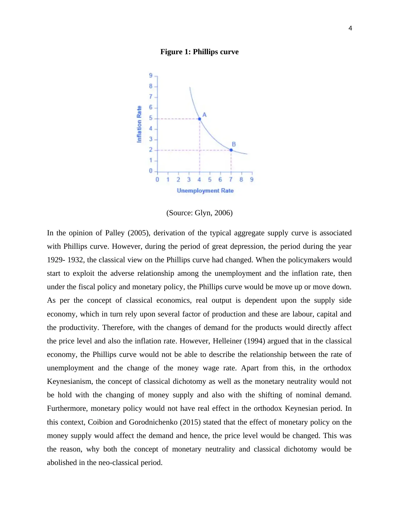
Figure 1: Phillips curve
(Source: Glyn, 2006)
In the opinion of Palley (2005), derivation of the typical aggregate supply curve is associated
with Phillips curve. However, during the period of great depression, the period during the year
1929- 1932, the classical view on the Phillips curve had changed. When the policymakers would
start to exploit the adverse relationship among the unemployment and the inflation rate, then
under the fiscal policy and monetary policy, the Phillips curve would be move up or move down.
As per the concept of classical economics, real output is dependent upon the supply side
economy, which in turn rely upon several factor of production and these are labour, capital and
the productivity. Therefore, with the changes of demand for the products would directly affect
the price level and also the inflation rate. However, Helleiner (1994) argued that in the classical
economy, the Phillips curve would not be able to describe the relationship between the rate of
unemployment and the change of the money wage rate. Apart from this, in the orthodox
Keynesianism, the concept of classical dichotomy as well as the monetary neutrality would not
be hold with the changing of money supply and also with the shifting of nominal demand.
Furthermore, monetary policy would not have real effect in the orthodox Keynesian period. In
this context, Coibion and Gorodnichenko (2015) stated that the effect of monetary policy on the
money supply would affect the demand and hence, the price level would be changed. This was
the reason, why both the concept of monetary neutrality and classical dichotomy would be
abolished in the neo-classical period.

5
In the neo-classical synthesis, it can be mentioned that the Phillips curve can establish the
relationship between the rates of inflation with the changing of the real economic activities.
However, this concept was against the concept of Phillips curve, which was found in the year
1958. In the orthodox Keynesian, the Phillips curve would formulate the statistical relationship
between the percentage changes in the nominal wage rate and the rate of unemployment. More
specifically, Phillips curve would derive an inverse association between the wage inflation and
the unemployment rate as the proxy of the relationship of price inflation and the real output of
the classical period. Therefore, aggregate supply (AS) curve has positive and finite slope, which
would be related with the negatively sloping Phillips curve. It would in turn develop a positive
relationship between the output level and the rate of inflation. In case of equilibrium position of
the labour market, then the nominal wage rate would not be changed. With the rise of aggregate
demand, it would increase the labour demand and hence, the rate of unemployment would be
declined below the level of equilibrium. Consequently, the nominal wage rate of the employees
and the price level would be increased. Therefore, Galí (2011) cited that the negative slope of the
Phillips curve is the reflection of the excess demand of labour and the lowering unemployment
rate. On the other hand, the wage inflation would also be increased. From this point, it can be
stated that the neoclassical synthesis is the effect of pre-Keynesian neoclassical theory as well as
the Keynesian macroeconomics. This theory was criticised by Richard Lipsey (1960) and stated
that the neoclassical micro theory was converted into the macroeconomics and was referred as
demand pull theories. He also stated that under the labour market disequilibrium position, wage
inflation is dependent upon the distinction among the labour demand and the supply of labour
(Gordon, 2011).
Expectations augmented Phillips curve
The expectations augmented Phillips curve has initiated adaptive expectations in the Phillips
curve. In the opinion of Correa and Minella (2010), the expectations augmented Phillips curve
was initially used for explaining the monetarist view. The expectations augmented model would
lead to the shift of government ability to act. Moreover, under the Keynesian money illusion, the
changes of nominal variables such as the price level and the wage rate as well as the purchasing
power would be stable. As a result, if the government would decide to rely on the expansionary
monetary policy, then the unemployment rate would be declined and the inflation rate would be

6
increased. On the other hand, both Phelps and Friedman had argued that the government would
not trade at the high rate of unemployment for lowering down the unemployment rate. Both the
economists mentioned that the real wage rate is constant. In this context, the government would
use both the fiscal or monetary policy in order to lowering down the rate of unemployment under
the natural rate. As a result, increase in demand would increase the price level compared to the
anticipation rate of the employees. For instance, in case of higher revenues, the organisations
would like to employ more employees at the similar wage rate. In case of rising of money wage
rate, the organisations would stop to supply more labours. This is the reason, why the rate of
unemployment would be declined. Furthermore, the purchasing power would be decreased with
the reduction of purchasing power. On the contrary, Daly and Hobijn (2014) argued that with the
passage of time, and in case of higher price inflation, the organisations would like to supply less
labour and would create pressure to maximise the wage rate in order to align with the inflation
rate. Therefore, it can be inferred that both the presence of price inflation and wage inflation
would sustain expansionary fiscal policies at the higher rate.
Both the economists, Phelps and Friedman, also highlighted the diversification among the long
run and short run Phillips curve. As per the concept of Phillips curve of 1960s, the average
inflation rate would be constant, where the inflation rate and the rate of unemployment are
inversely associated. However, with the changes of average inflation rate, the policymakers
would continuously try to push down the rate of unemployment below the natural rate (Correa
and Minella, 2010). Therefore, if the perception of the workers would be similar with the real
values, then the natural unemployment rate would be compatible with the inflation rate.
Therefore, the long run Phillips curve would be vertical and it would be above the natural rate.
Nonetheless, in the transitional phase, it can be observed that the average rate of inflation would
be shifted persistently (Mavroeidis, Plagborg-Møller and Stock, 2014). More specifically, it can
be stated that both the long run as well as short run is the combination of expectations augmented
Phillips curve. The unemployment rate would be returned to its natural rate when the expectation
of the workers towards the price inflation would adapt the changes of actual inflation rate.
On the contrary, Mavroeidis, Plagborg-Møller and Stock (2014) argued that the trade-off among
the unemployment rate and the inflation rate, which would be explained with the help of Phillips
curve, had broken down during the stagflationary period of 1970. During this period, both the

7
unemployment rate and the rate of inflation had been increased rapidly. As per the statement of
the monetarists, the rising of money supply would lead to increase the wage inflation and it
would not reduce the unemployment rate. As per the statement of Milton Friedman, the trade-off
relationship does not hold among the inflation rate and the unemployment rate in the long run.
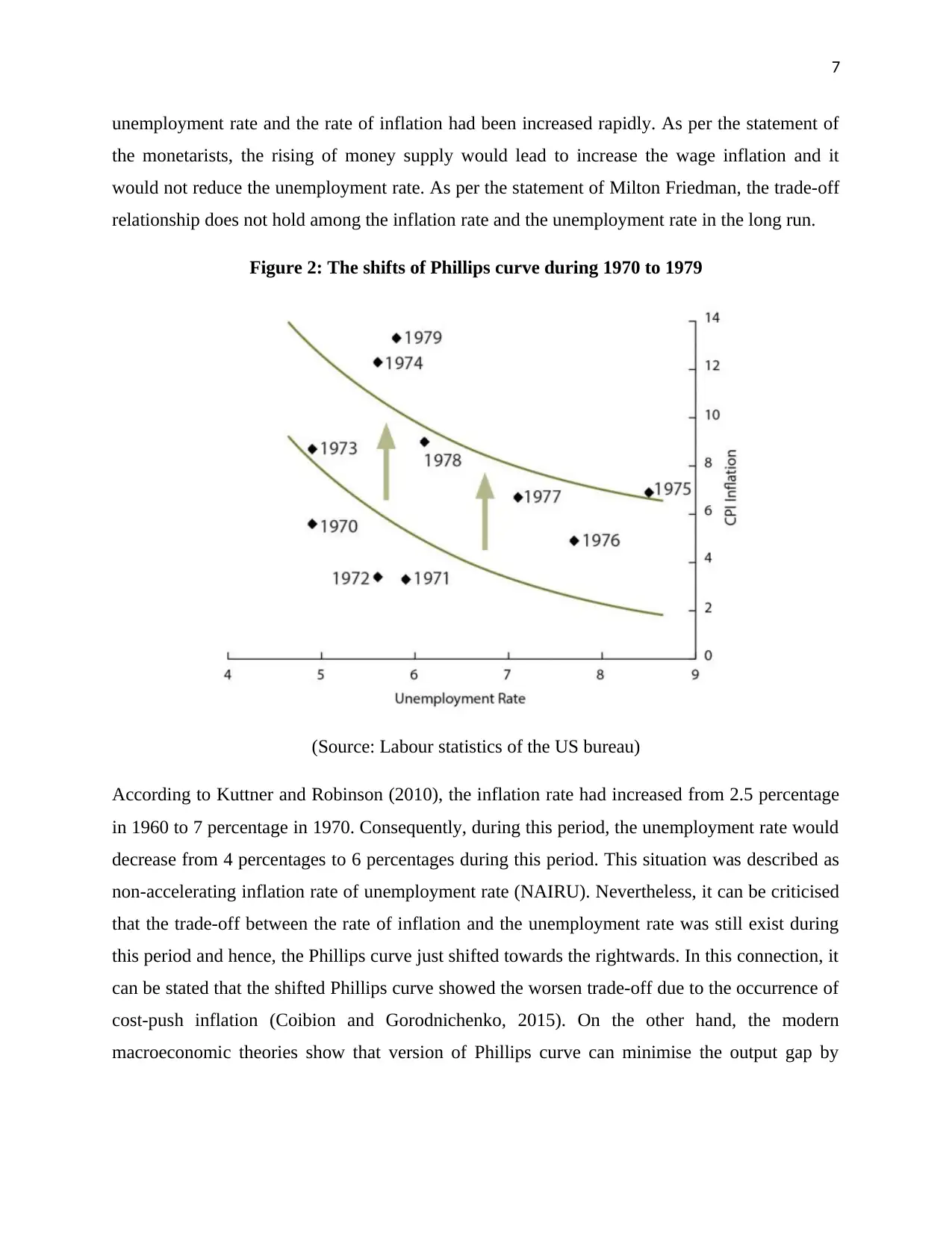
Figure 2: The shifts of Phillips curve during 1970 to 1979
(Source: Labour statistics of the US bureau)
According to Kuttner and Robinson (2010), the inflation rate had increased from 2.5 percentage
in 1960 to 7 percentage in 1970. Consequently, during this period, the unemployment rate would
decrease from 4 percentages to 6 percentages during this period. This situation was described as
non-accelerating inflation rate of unemployment rate (NAIRU). Nevertheless, it can be criticised
that the trade-off between the rate of inflation and the unemployment rate was still exist during
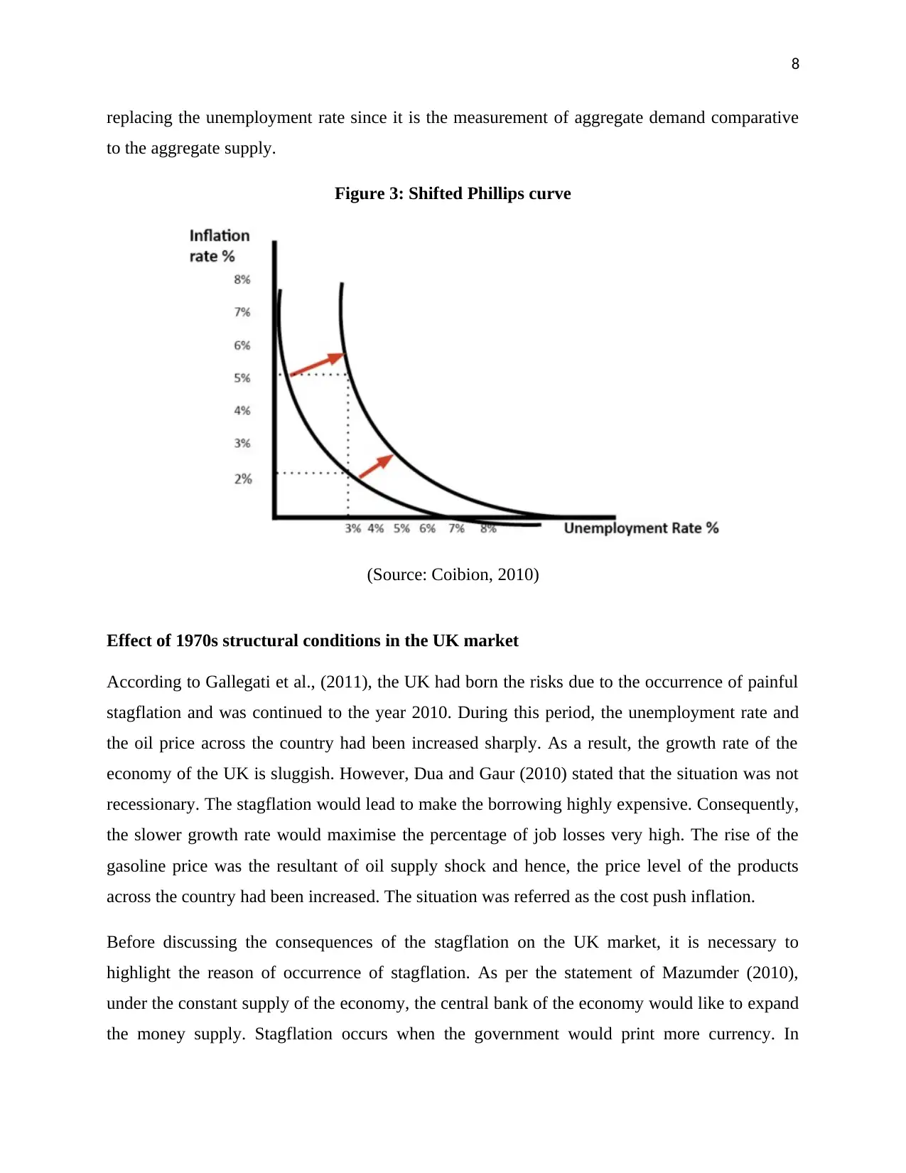
this period and hence, the Phillips curve just shifted towards the rightwards. In this connection, it
can be stated that the shifted Phillips curve showed the worsen trade-off due to the occurrence of
cost-push inflation (Coibion and Gorodnichenko, 2015). On the other hand, the modern
macroeconomic theories show that version of Phillips curve can minimise the output gap by

8
replacing the unemployment rate since it is the measurement of aggregate demand comparative
to the aggregate supply.
Figure 3: Shifted Phillips curve
(Source: Coibion, 2010)
Effect of 1970s structural conditions in the UK market
According to Gallegati et al., (2011), the UK had born the risks due to the occurrence of painful
stagflation and was continued to the year 2010. During this period, the unemployment rate and
the oil price across the country had been increased sharply. As a result, the growth rate of the
economy of the UK is sluggish. However, Dua and Gaur (2010) stated that the situation was not
recessionary. The stagflation would lead to make the borrowing highly expensive. Consequently,
the slower growth rate would maximise the percentage of job losses very high. The rise of the
gasoline price was the resultant of oil supply shock and hence, the price level of the products
across the country had been increased. The situation was referred as the cost push inflation.
Before discussing the consequences of the stagflation on the UK market, it is necessary to
highlight the reason of occurrence of stagflation. As per the statement of Mazumder (2010),
under the constant supply of the economy, the central bank of the economy would like to expand
the money supply. Stagflation occurs when the government would print more currency. In

9
addition, the central banks would aim to create more credit. Consequently, the money supply and
the money supply would be increased.
As per the concept of the Keynesian theories, the inflation rate is inversely related with the
unemployment rate as well as is positively related with the growth of the economy. In 1970, the
rising price level and the rising unemployment rate would be the resultant of cost push inflation
and hence, the oil price would be increased (Granger and Jeon, 2011). The monetary policy was
also expensive in this period. Apart from the monetary policy, the export and the import
behaviour of the country had been affected due to the stagflationary situation.
Effect of 1970s structural conditions in the international market place
It is known that stagflation occurs due to the higher inflation and the higher unemployment rate.
It prevents the growth rate of the economy. In the opinion of Jean-Baptiste (2012), after the
occurrence of the stagflation in 1970, the federal government had started to manipulate the
currency in order to spur the growth rate of the economy. The stagflation during the period of
1973 to 1975 was referred as the situation of recession. In the global economy, the
unemployment rate had reached to the highest peak in the year 1975 and was stuck at 9
percentages. The inflation rate also reached to 9.6 per cent from 3.4 per cent in 1973 (Rumler
and Valderrama, 2010; D'Arista, 2009). Apart from this, the global GDP was negative since last
three quarters of 1970.
During the stagflationary period, the US government had implemented three fiscal policies.
Firstly, Nixon, the US president of that period, had frozen the wage level and the price rate for
90 days. After that the price commission and pay board had developed for increasing the wage
and price after 90 days. This was beneficial to control the price level after the year of 1972. This
was the effective approach of controlling the global inflation rate. Secondly, Nixon had planned
to impose 10 percentage of tariff on the imports. He aimed at lowering down the balance of trade
for protecting the domestic firms. In addition, he increased the price of the importable. Thirdly,
Nixon had removed the system of gold standard. It would help to keep the value of dollar at the
fixed rate since the year 1944. In order to worsen the stagflation, the fed government had
increase the funds rate between the period of 1971to 1978 (Imbs, Jondeau and Pelgrin, 2011;

10
Snowdon and Vane, 2005). It had helped to increase the price level and hence, the inflation rate
has increased up to 13.3 percentages in the year of 1989.
Late 1960s and early 1970s theoretical and political crumbling of Keynesianism
As per the statement of Carlin and Soskice (1990), during the post war displacement period of
Keynesianism, the Keynesian economics would lead to develop developed world. The developed
world would be structured by the influence of economic policies, which had adopted by the
emerging countries. The policy makers were driven by the Keynesian thinking and followed the
free market policies instead of formulating the mixed economy since unnecessary government
intervention was required in this context. As a result, the world economy had been experiencing
a long boom by the prior period of 1970 (Glyn et al., 1986). In addition, in the year 1965, the
advanced capitalists countries had experienced persistent inflation rate.
Conclusion
Based on the analysis, it can be mentioned that the Phillips curve was derived based on stable
and inverse relationship of the inflation rate and the unemployment rate. This theory claims the
economic growth rate, which would in turn create more jobs, which would in turn reduce the
unemployment rate. However, as per the concept of expectation augmented Phillips curve, the
Phillips curve would not be sustained in the long run. Therefore, it can be inferred that the
Phillips curve would be broken down. On the other hand, Friedman also made a counter
argument and stated that in the long run, the Phillips curve would be shifted in the right ward.
Apart from this, based on the analysis it can be observed that during the stagflationary period of
1970, the trade-off among the unemployment rate and the inflation rate would be broken down
and hence, both the unemployment rate and the inflation rate had increased in this period.

11
Reference
Carlin, W. and Soskice, D., 1990. Macroeconomics and the wage bargain.
Coibion, O. and Gorodnichenko, Y., 2015. Is the Phillips curve alive and well after all? Inflation
expectations and the missing disinflation. American Economic Journal: Macroeconomics, 7(1),
pp.197-232.
Coibion, O., 2010. Testing the sticky information Phillips curve. The Review of Economics and
Statistics, 92(1), pp.87-101.
Colander, D., 1995. ‘The stories we tell: A reconsideration of AS/AD analysis’, Journal of
Economic Perspectives, 9(3): 169-188.
Correa, A.D.S. and Minella, A., 2010. Nonlinear mechanisms of the exchange rate pass-through:
A Phillips curve model with threshold for Brazil. Revista Brasileira de Economia, 64(3), pp.231-
243.
Daly, M.C. and Hobijn, B., 2014. Downward nominal wage rigidities bend the Phillips curve.
Journal of Money, Credit and Banking, 46(2), pp.51-93.
D'Arista, J., 2009. The evolving international monetary system. Cambridge Journal of
Economics, 33(4), pp.633-652.
Dua, P. and Gaur, U., 2010. Determination of inflation in an open economy Phillips curve
framework: The case of developed and developing Asian countries. Macroeconomics and
Finance in Emerging Market Economies, 3(1), pp.33-51.
Forder, J., 2010. ‘The historical place of the ‘Friedman-Phelps’ expectations critique’. European
Journal of Economic Thought. 17(2): 493-511.
Galí, J., 2011. The return of the wage Phillips curve. Journal of the European Economic
Association, 9(3), pp.436-461.

12
Gallegati, M., Gallegati, M., Ramsey, J.B. and Semmler, W., 2011. The US wage Phillips curve
across frequencies and over time. Oxford Bulletin of Economics and Statistics, 73(4), pp.489-
508.
Glyn, A., 2006. Chapters 1 & 2 in: Capitalism Unleashed. Finance, Globalization and Welfare,
Oxford: Oxford University Press.
Glyn, A., Hughes, A., Lipietz, A. and Singh, A., 1986. The Rise and Fall Of the Golden Age: an
historical analysis of post-war capitalism in the developed market economies. Marglin & Schor,
eds., The Golden Age of Capitalism.
Gordon, R.J., 2011. The history of the Phillips curve: Consensus and bifurcation. Economica,
78(3), pp.10-50.
Granger, C.W. and Jeon, Y., 2011. The evolution of the Phillips curve: a modern time series
viewpoint. Economica, 78(309), pp.51-66.
Helleiner, E., 1994. Chapters 4 & 5 in: States and the Reemergence of Global Finance. From
Bretton Woods to the 1990s, New York: Cornell Univeristy.
Imbs, J., Jondeau, E. and Pelgrin, F., 2011. Sectoral Phillips curves and the aggregate Phillips
curve. Journal of Monetary Economics, 58(4), pp.328-344.
Jean-Baptiste, F., 2012. Forecasting with the new Keynesian Phillips curve: Evidence from
survey data. Economics Letters, 117(3), pp.811-813.
Kuttner, K. and Robinson, T., 2010. Understanding the flattening Phillips curve. The North
American Journal of Economics and Finance, 21(2), pp.110-125.
Mavroeidis, S., Plagborg-Møller, M. and Stock, J.H., 2014. Empirical evidence on inflation
expectations in the New Keynesian Phillips Curve. Journal of Economic Literature, 52(1),
pp.124-88.
Mazumder, S., 2010. The new Keynesian Phillips curve and the cyclicality of marginal cost.
Journal of Macroeconomics, 32(3), pp.747-765.

13
Palley, T. I., 2005. ‘From Keynesianism to Neo-liberalism’ in: Saad-Filho, A. & D. Johnston
(eds.) Neo-liberalism A Critical Reader, London: Pluto Press 2005.
Rumler, F. and Valderrama, M.T., 2010. Comparing the New Keynesian Phillips Curve with
time series models to forecast inflation. The North American Journal of Economics and Finance,
21(2), pp.126-144.
Snowdon, B. and Vane, H.R., 2005. Modern macroeconomics: its origins, development and
current state. Edward Elgar Publishing.