1. INTRODUCTION TO ECONOMIC METHODS by Student’s Name.

1
INTRODUCTION TO ECONOMIC METHODS
by Student’s Name
Code + Name of Course
Professor’s Name
University
City (State)
Date

2
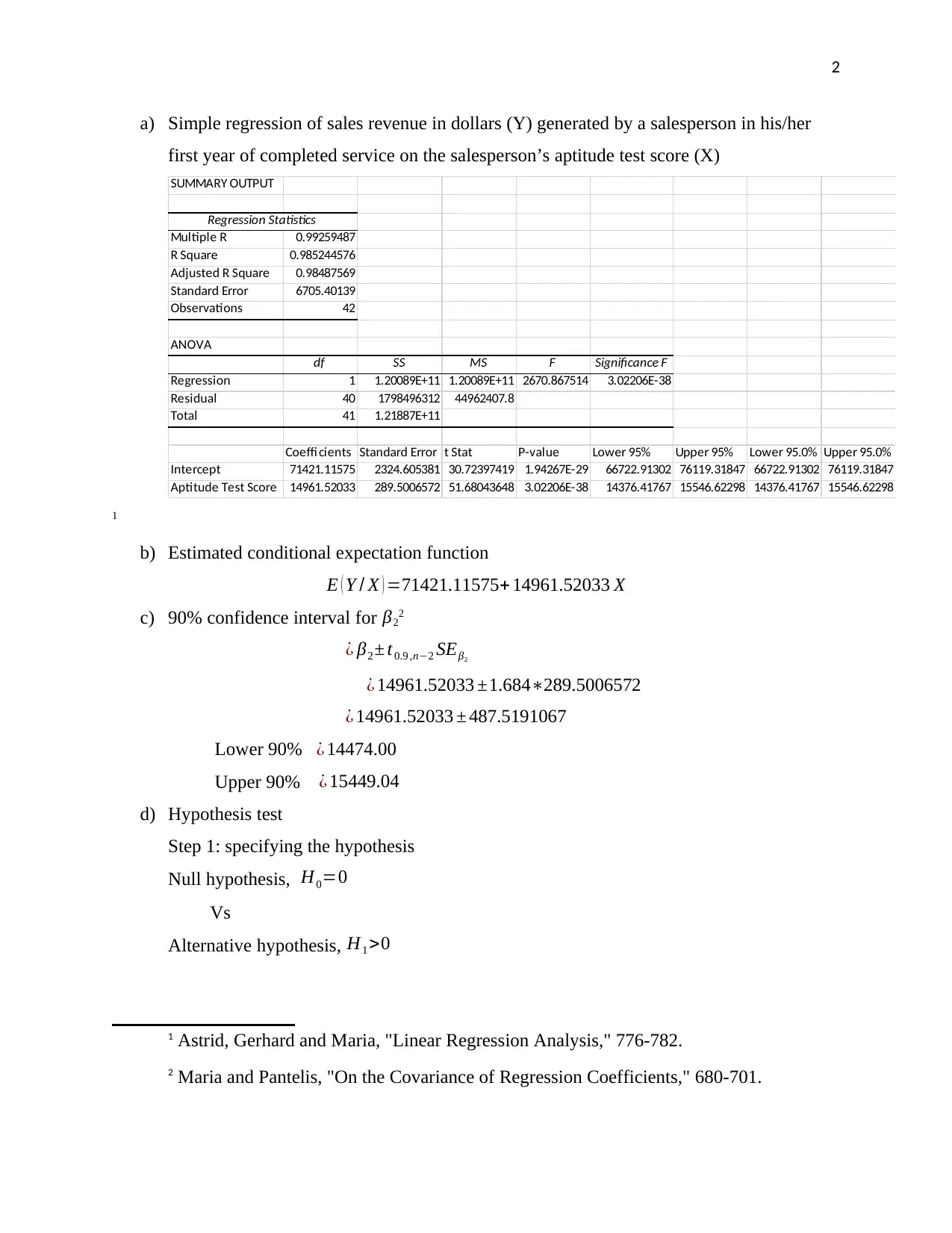
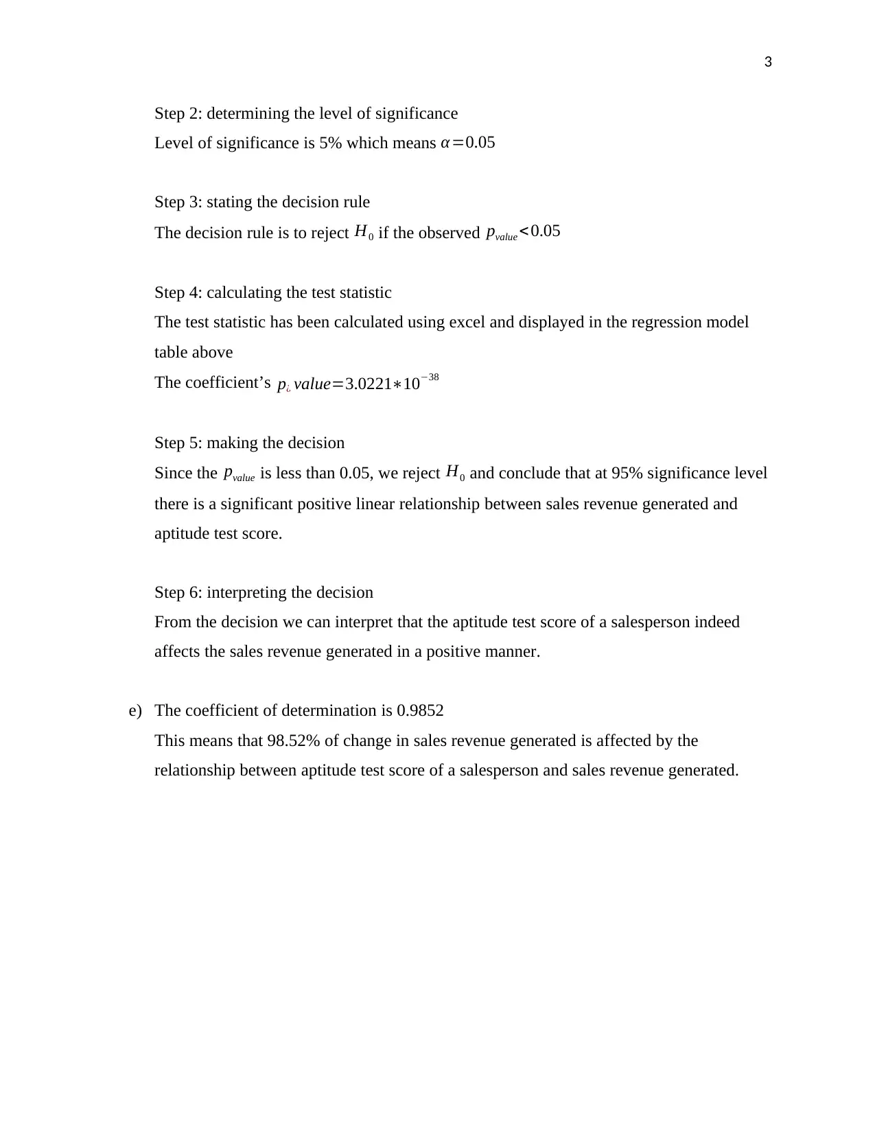
a) Simple regression of sales revenue in dollars (Y) generated by a salesperson in his/her
first year of completed service on the salesperson’s aptitude test score (X)
SUMMARY OUTPUT
Regression Statistics
Multiple R 0.99259487
R Square 0.985244576
Adjusted R Square 0.98487569
Standard Error 6705.40139
Observations 42
ANOVA
df SS MS F Significance F
Regression 1 1.20089E+11 1.20089E+11 2670.867514 3.02206E-38
Residual 40 1798496312 44962407.8
Total 41 1.21887E+11
Coeffi cients Standard Error t Stat P-value Lower 95% Upper 95% Lower 95.0% Upper 95.0%
Intercept 71421.11575 2324.605381 30.72397419 1.94267E-29 66722.91302 76119.31847 66722.91302 76119.31847
Aptitude Test Score 14961.52033 289.5006572 51.68043648 3.02206E-38 14376.41767 15546.62298 14376.41767 15546.62298
1
b) Estimated conditional expectation function
E ( Y / X ) =71421.11575+ 14961.52033 X
c) 90% confidence interval for β22
¿ β2 ± t0.9 ,n−2 SEβ2
¿ 14961.52033 ±1.684∗289.5006572
¿ 14961.52033 ± 487.5191067
Lower 90% ¿ 14474.00
Upper 90% ¿ 15449.04
d) Hypothesis test
Step 1: specifying the hypothesis
Null hypothesis, H0=0
Vs
Alternative hypothesis, H1 >0
1 Astrid, Gerhard and Maria, "Linear Regression Analysis," 776-782.
2 Maria and Pantelis, "On the Covariance of Regression Coefficients," 680-701.

3
Step 2: determining the level of significance
Level of significance is 5% which means α =0.05
Step 3: stating the decision rule
The decision rule is to reject H0 if the observed pvalue <0.05
Step 4: calculating the test statistic
The test statistic has been calculated using excel and displayed in the regression model
table above
The coefficient’s p¿ value=3.0221∗10−38
Step 5: making the decision
Since the pvalue is less than 0.05, we reject H0 and conclude that at 95% significance level
there is a significant positive linear relationship between sales revenue generated and
aptitude test score.
Step 6: interpreting the decision
From the decision we can interpret that the aptitude test score of a salesperson indeed
affects the sales revenue generated in a positive manner.
e) The coefficient of determination is 0.9852
This means that 98.52% of change in sales revenue generated is affected by the
relationship between aptitude test score of a salesperson and sales revenue generated.

4
References
Astrid, Gerhard, and Maria. 2010. "Linear Regression Analysis." Dtsch Arztebl Int 107(44), 776-782.
Maria, and Pantelis. 2015. "On the Covariance of Regression Coefficients." Journal of Statistics 5(7), 680-
701.