Inventory Management Assignment: Optimization and Cost Analysis

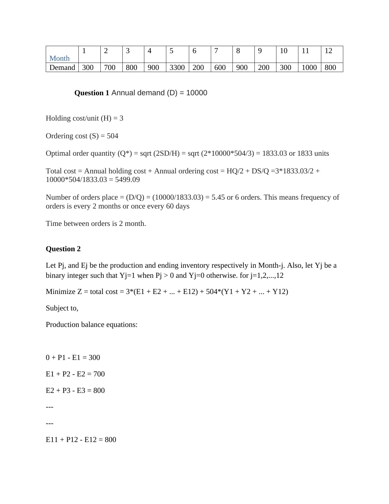
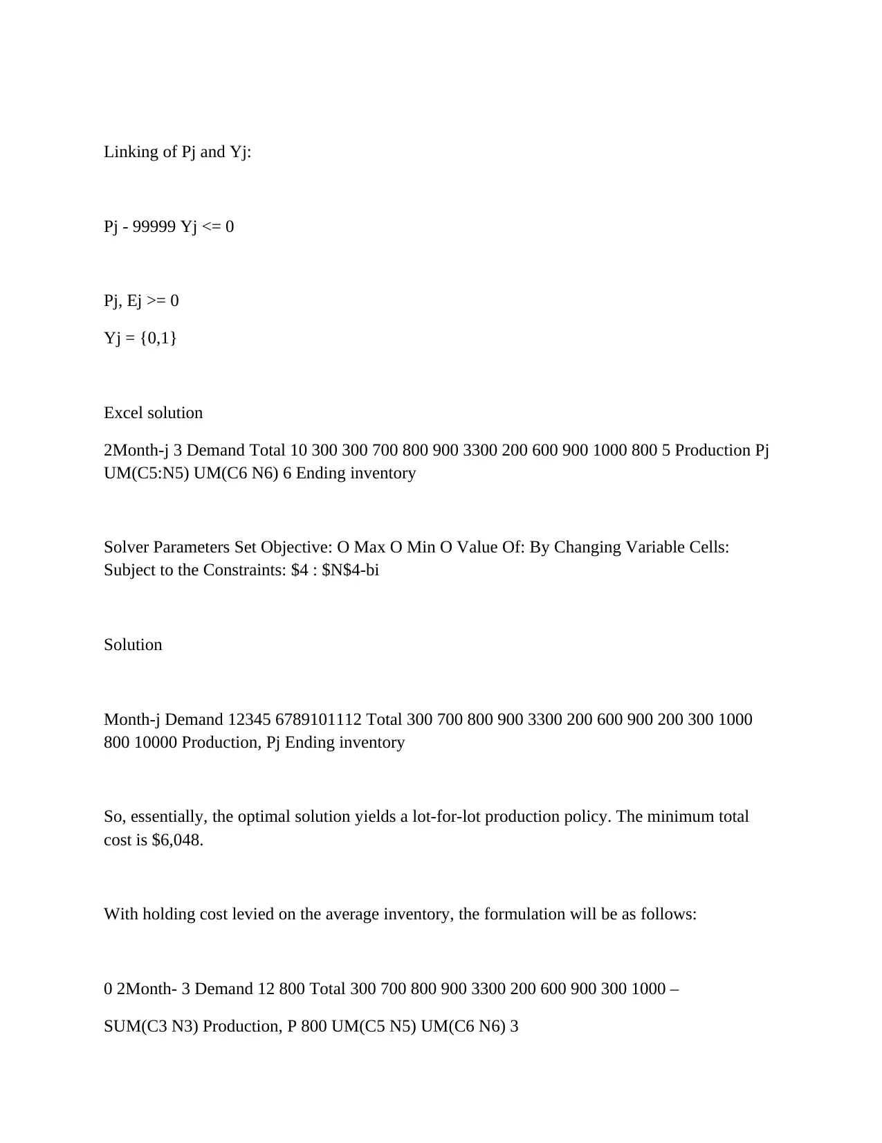
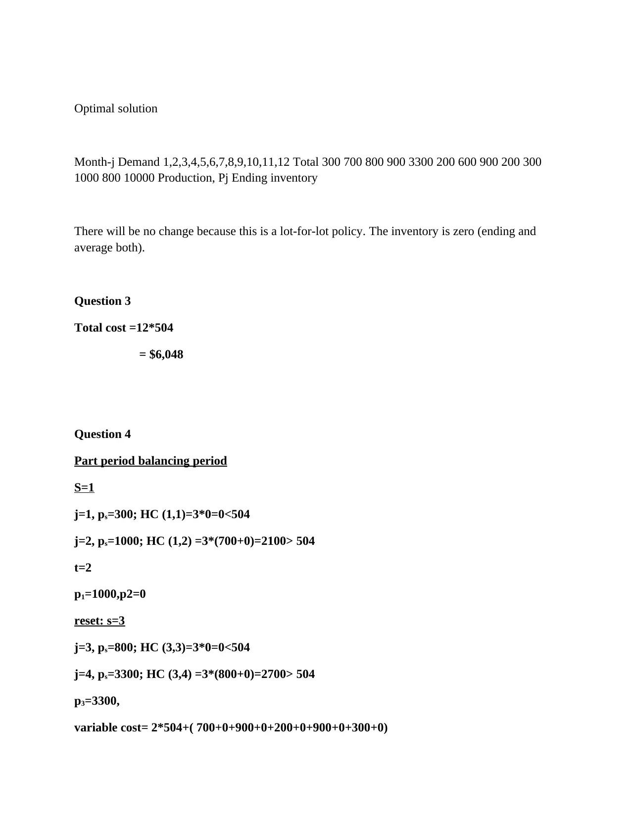
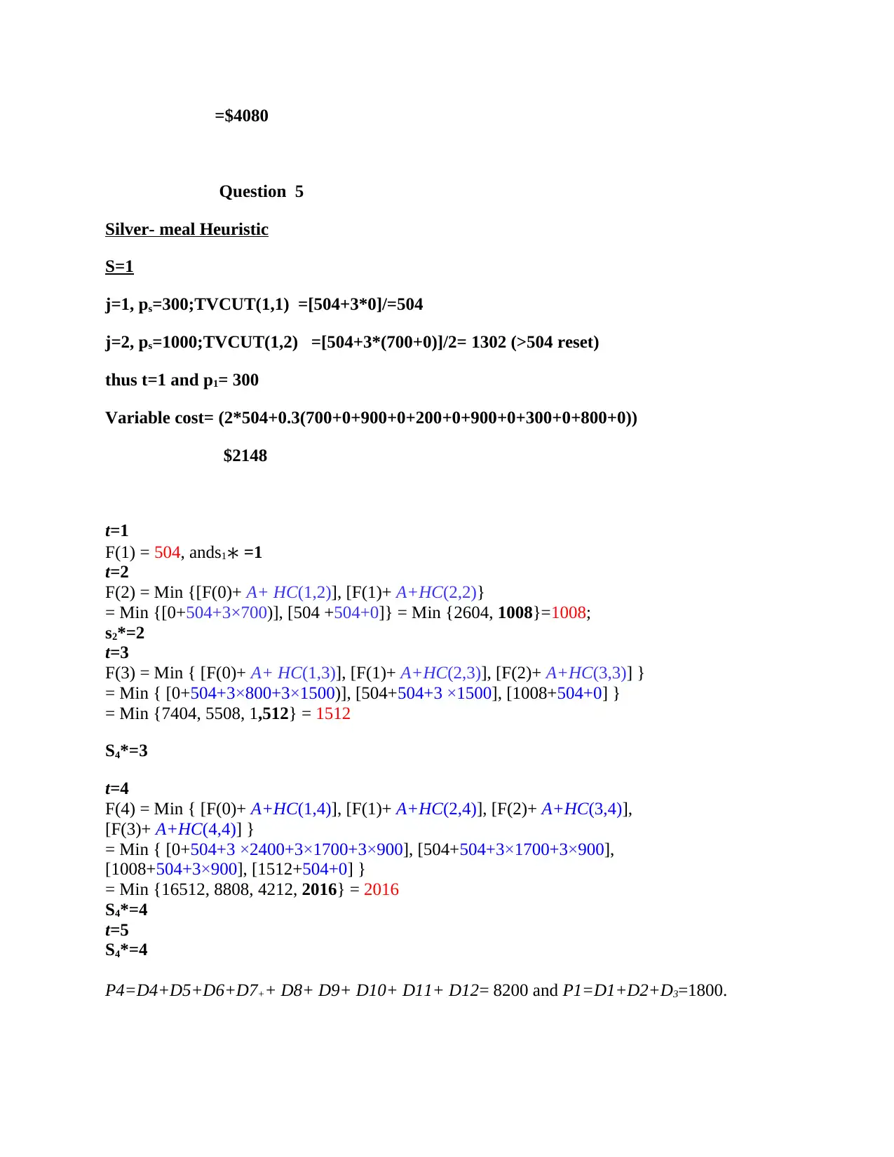
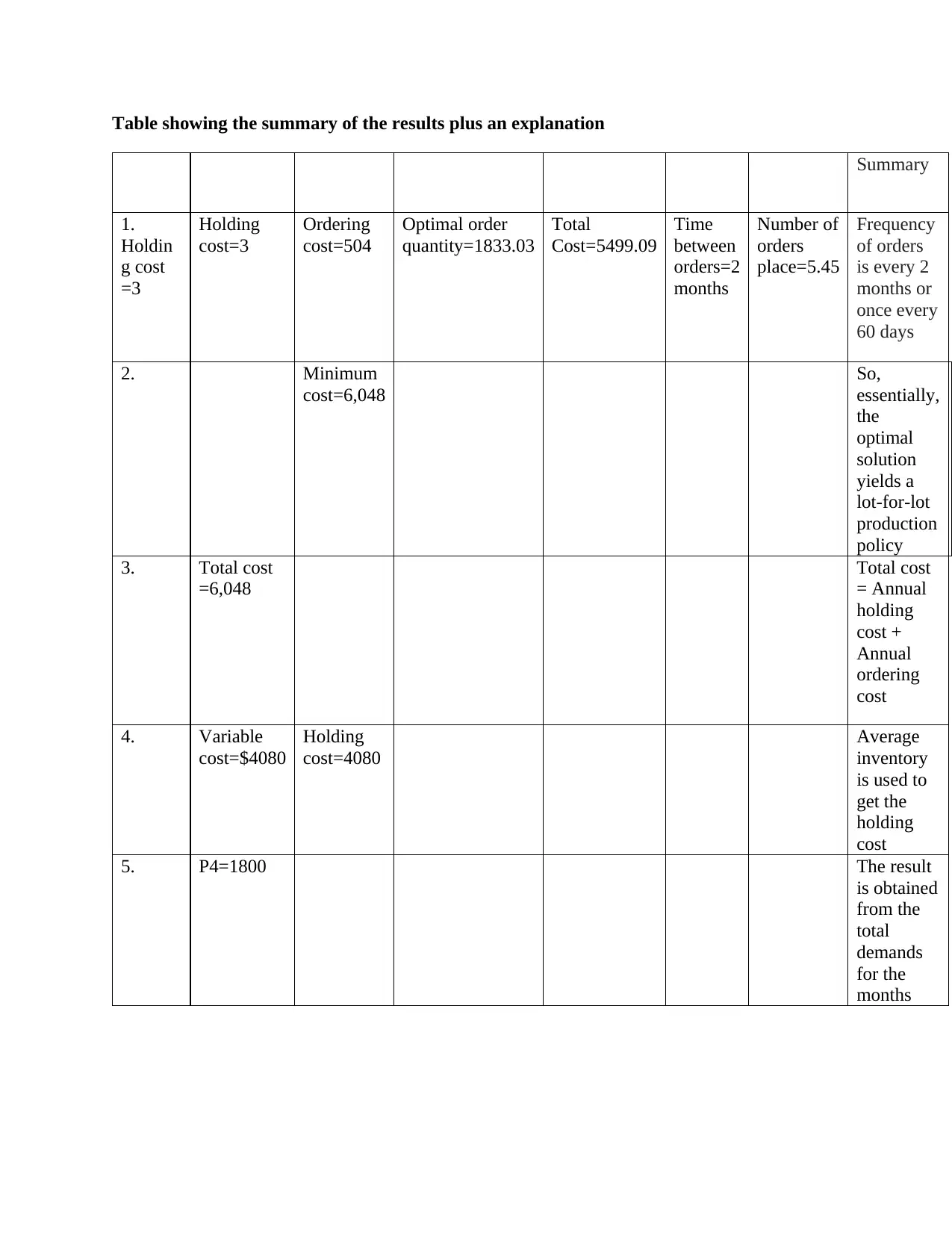
This assignment solution addresses an inventory management problem, calculating the optimal order quantity (1833 units) and total cost ($5499.09) using the Economic Order Quantity (EOQ) model. It analyzes annual demand, holding costs, and ordering costs. The solution then formulates a product...Read More

Month 1 2 3 4 5 6 7 8 9 10 11 12
Demand 300 700 800 900 3300 200 600 900 200 300 1000 800
Question 1 Annual demand (D) = 10000
Holding cost/unit (H) = 3
Ordering cost (S) = 504
Optimal order quantity (Q*) = sqrt (2SD/H) = sqrt (2*10000*504/3) = 1833.03 or 1833 units
Total cost = Annual holding cost + Annual ordering cost = HQ/2 + DS/Q =3*1833.03/2 +
10000*504/1833.03 = 5499.09
Number of orders place = (D/Q) = (10000/1833.03) = 5.45 or 6 orders. This means frequency of
orders is every 2 months or once every 60 days
Time between orders is 2 month.
Question 2
Let Pj, and Ej be the production and ending inventory respectively in Month-j. Also, let Yj be a
binary integer such that Yj=1 when Pj > 0 and Yj=0 otherwise. for j=1,2,...,12
Minimize Z = total cost = 3*(E1 + E2 + ... + E12) + 504*(Y1 + Y2 + ... + Y12)
Subject to,
Production balance equations:
0 + P1 - E1 = 300
E1 + P2 - E2 = 700
E2 + P3 - E3 = 800
---
---
E11 + P12 - E12 = 800

Linking of Pj and Yj:
Pj - 99999 Yj <= 0
Pj, Ej >= 0
Yj = {0,1}
Excel solution
2Month-j 3 Demand Total 10 300 300 700 800 900 3300 200 600 900 1000 800 5 Production Pj
UM(C5:N5) UM(C6 N6) 6 Ending inventory
Solver Parameters Set Objective: O Max O Min O Value Of: By Changing Variable Cells:
Subject to the Constraints: $4 : $N$4-bi
Solution
Month-j Demand 12345 6789101112 Total 300 700 800 900 3300 200 600 900 200 300 1000
800 10000 Production, Pj Ending inventory
So, essentially, the optimal solution yields a lot-for-lot production policy. The minimum total
cost is $6,048.
With holding cost levied on the average inventory, the formulation will be as follows:
0 2Month- 3 Demand 12 800 Total 300 700 800 900 3300 200 600 900 300 1000 –
SUM(C3 N3) Production, P 800 UM(C5 N5) UM(C6 N6) 3

Optimal solution
Month-j Demand 1,2,3,4,5,6,7,8,9,10,11,12 Total 300 700 800 900 3300 200 600 900 200 300
1000 800 10000 Production, Pj Ending inventory
There will be no change because this is a lot-for-lot policy. The inventory is zero (ending and
average both).
Question 3
Total cost =12*504
= $6,048
Question 4
Part period balancing period
S=1
j=1, ps=300; HC (1,1)=3*0=0<504
j=2, ps=1000; HC (1,2) =3*(700+0)=2100> 504
t=2
p1=1000,p2=0
reset: s=3
j=3, ps=800; HC (3,3)=3*0=0<504
j=4, ps=3300; HC (3,4) =3*(800+0)=2700> 504
p3=3300,
variable cost= 2*504+( 700+0+900+0+200+0+900+0+300+0)

=$4080
Question 5
Silver- meal Heuristic
S=1
j=1, ps=300;TVCUT(1,1) =[504+3*0]/=504
j=2, ps=1000;TVCUT(1,2) =[504+3*(700+0)]/2= 1302 (>504 reset)
thus t=1 and p1= 300
Variable cost= (2*504+0.3(700+0+900+0+200+0+900+0+300+0+800+0))
$2148
t=1
F(1) = 504, ands1∗ =1
t=2
F(2) = Min {[F(0)+ A+ HC(1,2)], [F(1)+ A+HC(2,2)}
= Min {[0+504+3×700)], [504 +504+0]} = Min {2604, 1008}=1008;
s2*=2
t=3
F(3) = Min { [F(0)+ A+ HC(1,3)], [F(1)+ A+HC(2,3)], [F(2)+ A+HC(3,3)] }
= Min { [0+504+3×800+3×1500)], [504+504+3 ×1500], [1008+504+0] }
= Min {7404, 5508, 1,512} = 1512
S4*=3
t=4
F(4) = Min { [F(0)+ A+HC(1,4)], [F(1)+ A+HC(2,4)], [F(2)+ A+HC(3,4)],
[F(3)+ A+HC(4,4)] }
= Min { [0+504+3 ×2400+3×1700+3×900], [504+504+3×1700+3×900],
[1008+504+3×900], [1512+504+0] }
= Min {16512, 8808, 4212, 2016} = 2016
S4*=4
t=5
S4*=4
P4=D4+D5+D6+D7++ D8+ D9+ D10+ D11+ D12= 8200 and P1=D1+D2+D3=1800.

Table showing the summary of the results plus an explanation
Summary
1.
Holdin
g cost
=3
Holding
cost=3
Ordering
cost=504
Optimal order
quantity=1833.03
Total
Cost=5499.09
Time
between
orders=2
months
Number of
orders
place=5.45
Frequency
of orders
is every 2
months or
once every
60 days
2. Minimum
cost=6,048
So,
essentially,
the
optimal
solution
yields a
lot-for-lot
production
policy
3. Total cost
=6,048
Total cost
= Annual
holding
cost +
Annual
ordering
cost
4. Variable
cost=$4080
Holding
cost=4080
Average
inventory
is used to
get the
holding
cost
5. P4=1800 The result
is obtained
from the
total
demands
for the
months

References
Axsater, S.(2006). Inventory control. Second Edition, MA: Springer US International Series in
operations research and management science).
Gorham, T.(1998) ‘Dynamic order quantities, ’Production and Inventory Management,9(1),
pp.75-81