Probability & Statistics

This document contains solved problems related to Probability & Statistics. It covers topics such as sufficient statistics, maximum likelihood estimation, biasness, and more.

1
PROBABILITY & STATISTICS
Student’s Name:
University Affiliate:
Course:
Problem 6.1.7

2
L(X1,,…….,Xn)=(2pi σ2)-n/2exp(-1/2σ2)∑ni=1(xi-u)2)
=(2piσ2)-n/2exp(-n/2σ2(ẋ-u)2exp(-n-1/2σ2s2)
=Hence(ẋ,s2) is a sufficient statistic.
When μ is fixed at ẋ, we get,
L((ẋ,σ2)|x1,……,xn)=2 πσ2)-n/2exp(n-1/2σ2s2)
Maximized as a function of σ2
Therefore,
{ӘlnL((ẋ,σ2)|x)}/Әσ2=Ә/Әσ2(-n/2Inσ2-n-1/2σ2s2)
=-n/2σ2+(n-1/2σ4)s2
Problem 6.1.19
T(x) is a minimal sufficient statistic if and only if;
fθ(x)/fθ(x) is independent of θ ͢͢ T(x)=T(y) as a consequence of Fisher’s
factorization theorem.
Gamma fθ(x)=θα0/┌(α0)xα0-1eβx
fθ(Xn)/fθ(yn)=(∏ni=1θα0/┌(α0)xα0-1e-βxi)/(∏ni=1βα0/┌(α0)yα0-1e-βyi)
=(∏ni=1(xi)αo-1(∏ni=1yi)α0-1e∑xi/e∑yi
=(∏ni=1xi/∏ni=1yi)α-1e(∑yi-∑xi
=The minimum sufficient statistic for (α,θ)=(∏xi-∑ni=1xi
Problem 6.1.11
L(θ|X0)=θx0 =1
∫10L(θ|X0) =0
The likelihood is a constant, hence the integral of a constant is 0.
Problem 6.2.4
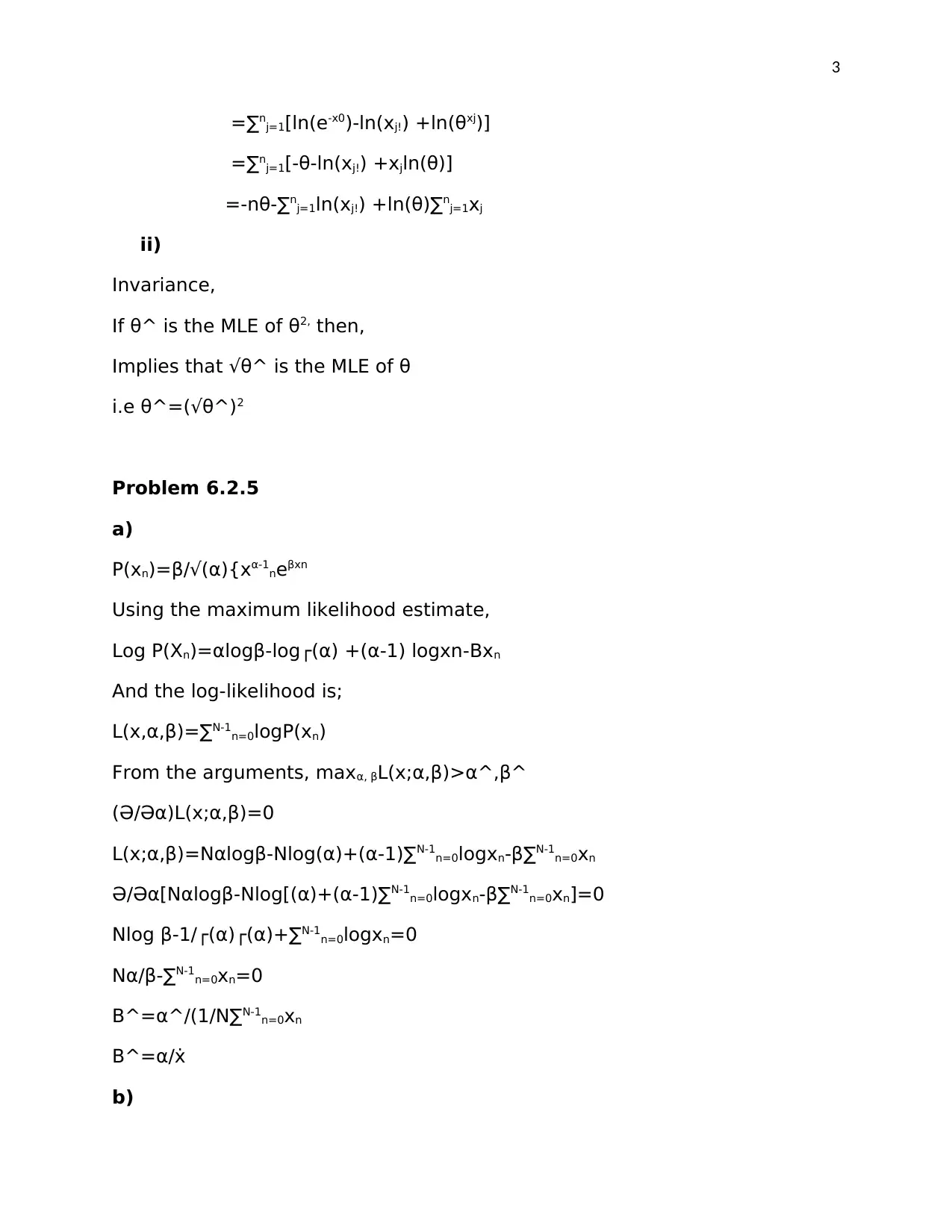
i) L(θ;x1,,……xn)=ln(∏nj=1exp(-θ2)1/xj!θ2xj
=- ∑nj=1ln(exp(-θ2)

3
=∑nj=1[ln(e-x0)-ln(xj!) +ln(θxj)]
=∑nj=1[-θ-ln(xj!) +xjln(θ)]
=-nθ-∑nj=1ln(xj!) +ln(θ)∑nj=1xj
ii)
Invariance,
If θ^ is the MLE of θ2, then,
Implies that √θ^ is the MLE of θ
i.e θ^=(√θ^)2
Problem 6.2.5
a)
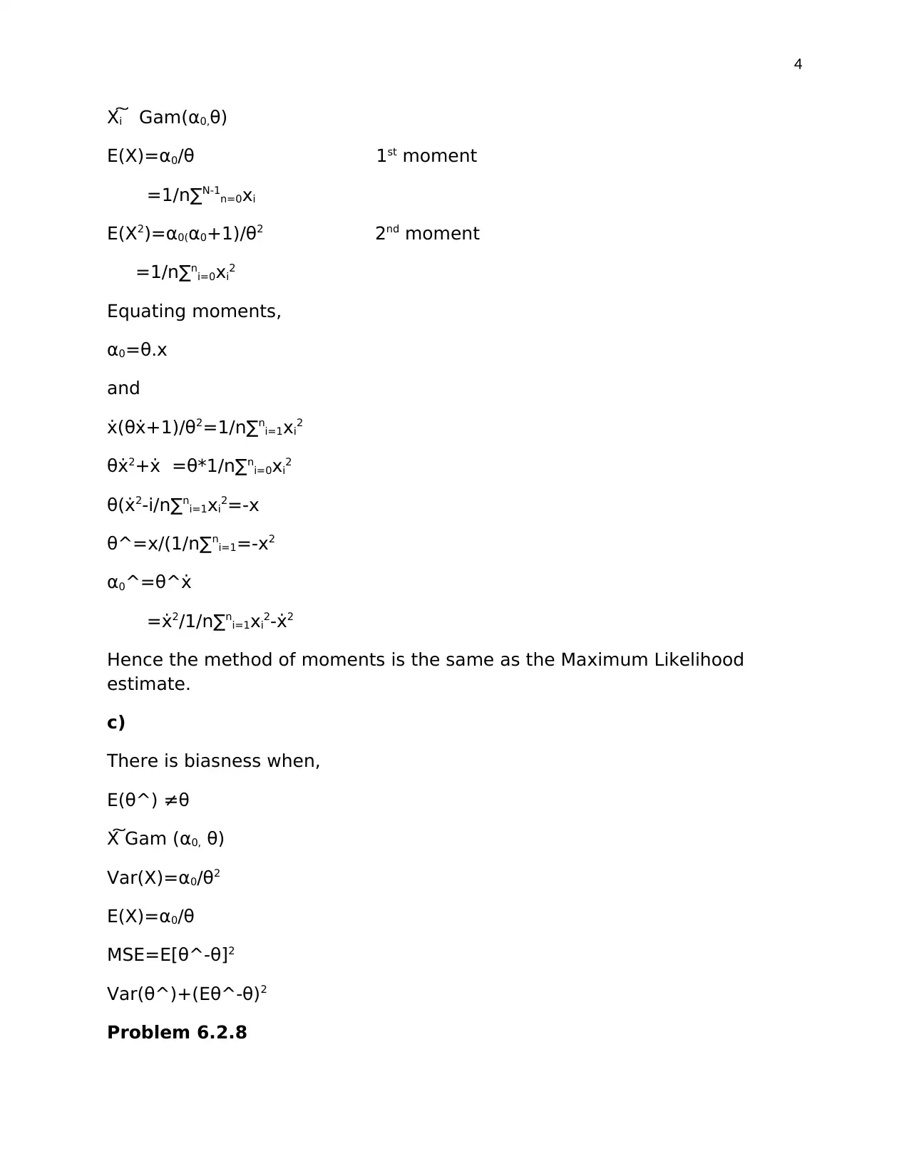
P(xn)=β/√(α){xα-1neβxn
Using the maximum likelihood estimate,
Log P(Xn)=αlogβ-log┌(α) +(α-1) logxn-Bxn
And the log-likelihood is;
L(x,α,β)=∑N-1n=0logP(xn)
From the arguments, maxα, βL(x;α,β)>α^,β^
(Ә/Әα)L(x;α,β)=0
L(x;α,β)=Nαlogβ-Nlog(α)+(α-1)∑N-1n=0logxn-β∑N-1n=0xn
Ә/Әα[Nαlogβ-Nlog[(α)+(α-1)∑N-1n=0logxn-β∑N-1n=0xn]=0
Nlog β-1/┌(α)┌(α)+∑N-1n=0logxn=0
Nα/β-∑N-1n=0xn=0
Β^=α^/(1/N∑N-1n=0xn
Β^=α/ẋ
b)

4
Xi͠ Gam(α0,θ)
E(X)=α0/θ 1st moment
=1/n∑N-1n=0xi
E(X2)=α0(α0+1)/θ2 2nd moment
=1/n∑ni=0xi2
Equating moments,
α0=θ.x
and
ẋ(θẋ+1)/θ2=1/n∑ni=1xi2
θẋ2+ẋ =θ*1/n∑ni=0xi2
θ(ẋ2-i/n∑ni=1xi2=-x
θ^=x/(1/n∑ni=1=-x2
α0^=θ^ẋ
=ẋ2/1/n∑ni=1xi2-ẋ2
Hence the method of moments is the same as the Maximum Likelihood
estimate.
c)
There is biasness when,
E(θ^) ≠θ
X͠ Gam (α0, θ)
Var(X)=α0/θ2
E(X)=α0/θ
MSE=E[θ^-θ]2
Var(θ^)+(Eθ^-θ)2
Problem 6.2.8

5
L(X1,,……,Xn,θ)=∏fθ(xi)
Which when maximized gives;
L(X1,…..Xn,θ^)=supθ{∏ni=1fθ(xi)}
(Ә/Әθ)∏ni=1fθ(xi)=0
However, differentiating might be so cumbersome.
Alternatively;
When we maximize the log of likelihood, we get,
L(x1,…….xn,θ)=log(L(x1,,…..xn,θ)
=∑i=1nlog(fθ(xi)
L(x1,,……xn,θ^)=supθ{∑ni=0log(fθ(xi)}
Ә/Әθjl(x1,,,….Xn,θ^)=Ә/Әθj∑ni=1log(fθ(xi))
∑ni=0Ә/Әθjlog(fθ(xi)=0
Problem 6.2.12.
a)
L=F(x2,x2,…xn|θ)=f(x1|θ)*f(x2|θ)*………*f(xn|θ)
And the log –likelihood function is;
L^=1/nlogL=1/n∑ni=1logf(xi|θ)
The plug-in MLE of σ2 is identical to the likelihood function.
b)
E[s2]=E[1/n∑ni=0(Xi-μ)2-2/n(ẋ-μ)∑ni=1(xi-μ)+(ẋ)-μ)2]
=E(1/n∑ni=1(xi-μ)2-2/n(ẋ-μ).n.(ẋ-μ)+(ẋ-μ)2
=E[1/n∑ni=1(Xi-μ)2-(ẋ-μ)2
=E[1/n∑ni=0(xi-μ)-E[ẋ-μ)2]
=σ2-E[ẋ-μ)2]=(1-1/n)σ2<σ2
MSE(θ^)=Eθ[(θ^-θ)2]

6
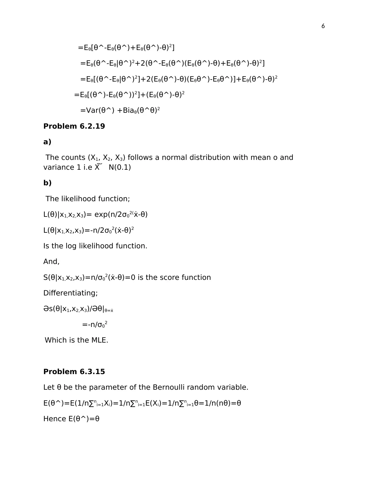
=Eθ[θ^-Eθ(θ^)+Eθ(θ^)-θ)2]
=Eθ(θ^-Eθ|θ^)2+2(θ^-Eθ(θ^)(Eθ(θ^)-θ)+Eθ(θ^)-θ)2]
=Eθ[(θ^-Eθ|θ^)2]+2(Eθ(θ^)-θ)(Eθθ^)-Eθθ^)]+Eθ(θ^)-θ)2
=Eθ[(θ^)-Eθ(θ^))2]+(Eθ(θ^)-θ)2
=Var(θ^) +Biaθ(θ^θ)2
Problem 6.2.19
a)
The counts (X1, X2, X3) follows a normal distribution with mean o and
variance 1 i.e X͠ N(0.1)
b)
The likelihood function;
L(θ)|x1,x2,x3)= exp(n/2σ02(ẋ-θ)
L(θ|x1,x2,x3)=-n/2σ02(ẋ-θ)2
Is the log likelihood function.
And,
S(θ|x1,x2,x3)=n/σ02(ẋ-θ)=0 is the score function
Differentiating;
Әs(θ|x1,x2,x3)/Әθ|θ=ẋ
=-n/σ02
Which is the MLE.
Problem 6.3.15
Let θ be the parameter of the Bernoulli random variable.
E(θ^)=E(1/n∑ni=1Xi)=1/n∑ni=1E(Xi)=1/n∑ni=1θ=1/n(nθ)=θ
Hence E(θ^)=θ

7
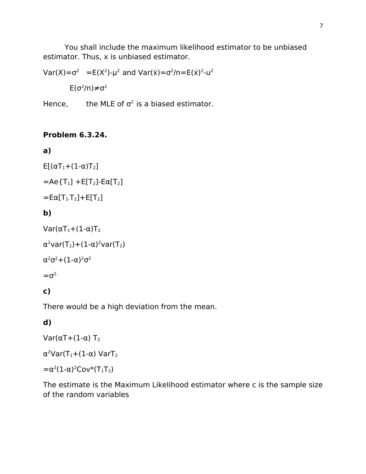
You shall include the maximum likelihood estimator to be unbiased
estimator. Thus, x is unbiased estimator.
Var(X)=σ2 =E(X2)-μ2 and Var(ẋ)=σ2/n=E(ẋ)2-u2
E(σ2/n)≠σ2
Hence, the MLE of σ2 is a biased estimator.
Problem 6.3.24.
a)
E[(αT1+(1-α)T2]
=Αe{T1] +E[T2]-Eα[T2]
=Eα[T1-T2]+E[T2]
b)
Var(αT1+(1-α)T2
α2var(T1)+(1-α)2var(T2)
α2σ2+(1-α)2σ2
=σ2.
c)
There would be a high deviation from the mean.
d)
Var(αT+(1-α) T2
α2Var(T1+(1-α) VarT2
=α2(1-α)2Cov*(T1T2)
The estimate is the Maximum Likelihood estimator where c is the sample size
of the random variables

8
References:
Windmeijer, F., 2005. A finite sample correction for the variance of linear
efficient two-step GMM estimators. Journal of econometrics, 126(1), pp.25-
51.