HA1011 Applied Quantitative Methods: Business Statistics Assignment
VerifiedAdded on 2023/04/04
|10
|1073
|193
Homework Assignment
AI Summary
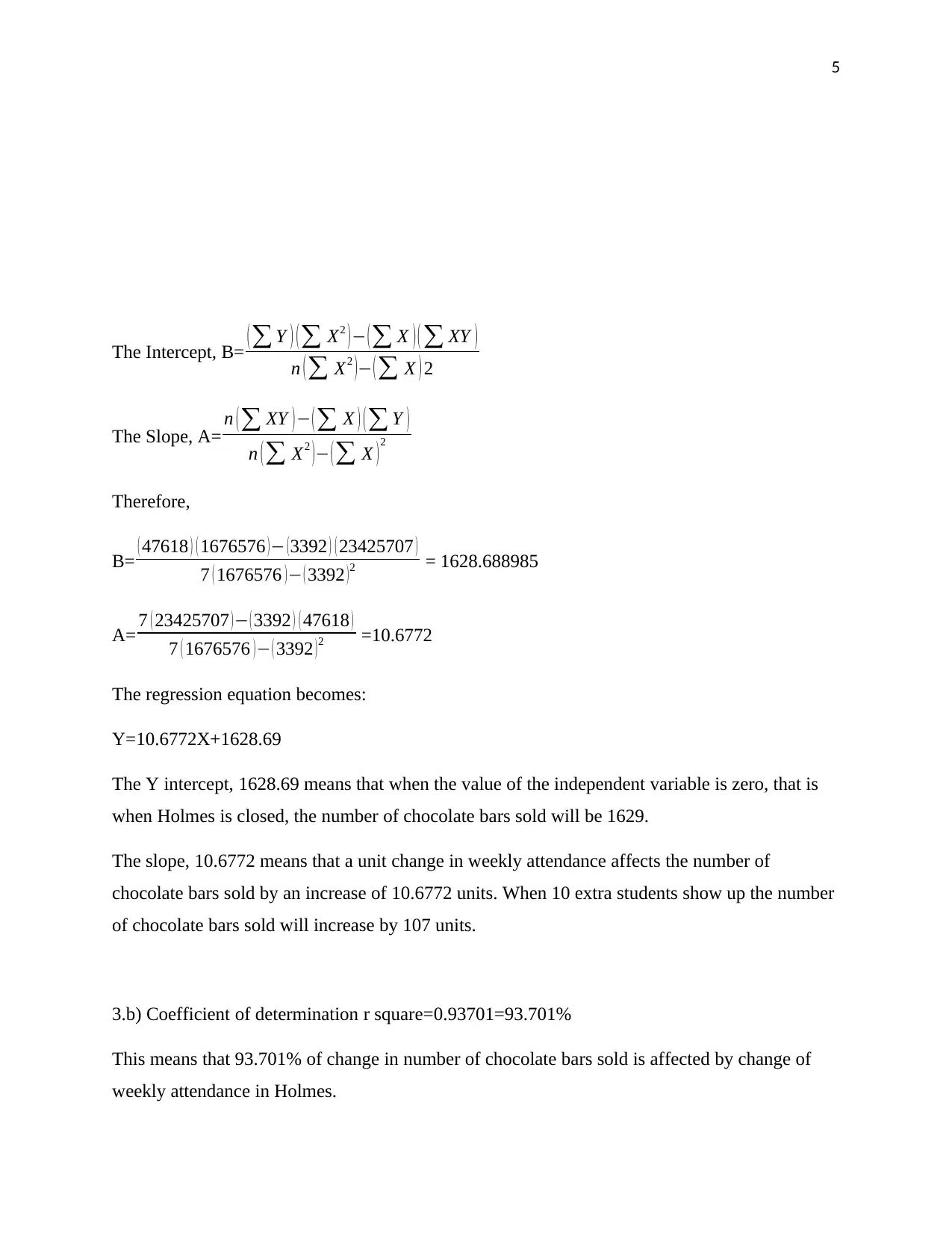
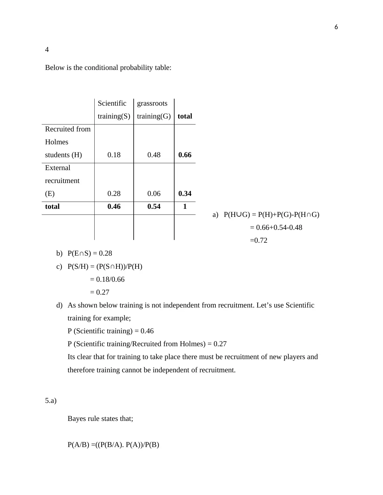
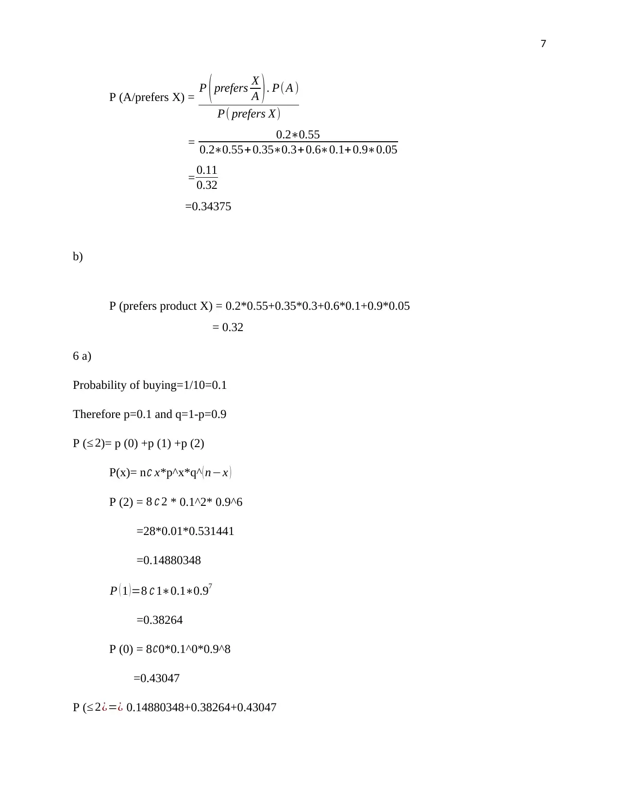
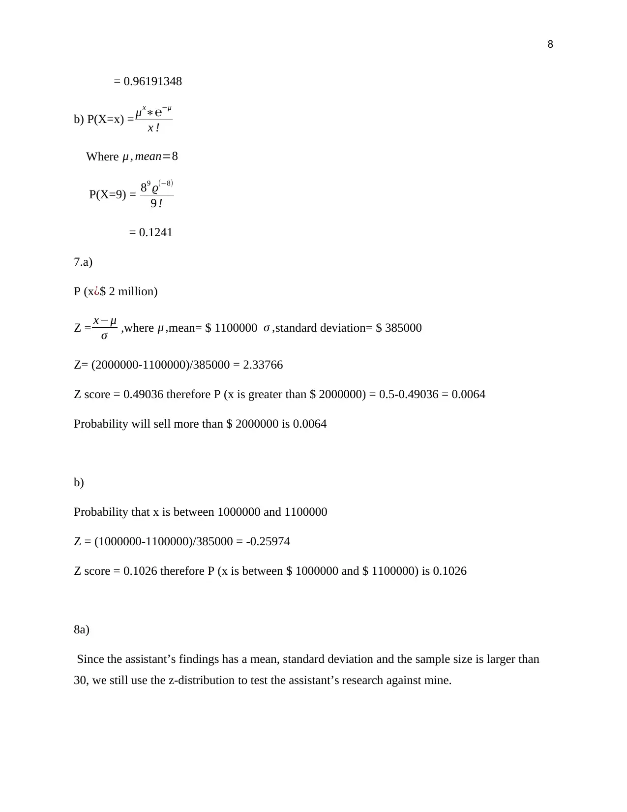
This assignment solution covers various statistical concepts applied to business scenarios. It includes creating frequency distributions, calculating mean, median, and mode, and interpreting standard deviation and interquartile range. The solution also addresses correlation analysis between weekly attendance and chocolate bar sales, constructing a regression equation, and applying conditional probability and Bayes' rule. Furthermore, it involves binomial and Poisson probability calculations, along with normal distribution problems related to sales projections. The assignment concludes with hypothesis testing and probability calculations related to investor commitment. Desklib offers a wealth of similar solved assignments and study resources for students.

1
STATISTICS FOR BUSINESS
by Student’s Name
Code + Name of Course
Professor’s Name
University
City(state)
Date
STATISTICS FOR BUSINESS
by Student’s Name
Code + Name of Course
Professor’s Name
University
City(state)
Date
Paraphrase This Document
Need a fresh take? Get an instant paraphrase of this document with our AI Paraphraser

2
1.a)
bins Frequency
Relative
frequency
cumulative
frequency
cumulative
relative
frequency
Class
midpoint
300 6 10.00% 6 10.00% 150
600 18 30.00% 24 40.00% 450
900 9 15.00% 33 55.00% 750
1200 11 18.33% 44 73.33% 1050
1500 4 6.67% 48 80.00% 1350
1800 5 8.33% 53 88.33% 1650
2100 2 3.33% 55 91.67% 1950
2400 1 1.67% 56 93.33% 2250
2700 1 1.67% 57 95.00% 2550
3000 2 3.33% 59 98.33% 2850
3300 1 1.67% 60 100.00% 3150
1.b)
0
2
4
6
8
10
12
14
16
18
20
300
600
900
1200
1500
1800
2100
2400
2700
3000
3300
More
Frequency
Bin
Histogram
Frequency
1.c)
Mean 976.5667
Median 797.5
Mode 401

3
2.a)
The data set is a sample because it’s only observed during a short period of time, that is a
few number of weeks that the supermarket has and will be in operation. A population would
otherwise be observed during the entire time the supermarket will be in operation.
2.b)
Standard deviation, δ= √ ∑ ( x−μ ) 2
n−1
weekly
attendance
(X) x-μ (x-μ)^2
472 472-484.57=-12.57 158.0049
413 413-484.57=-71.57 5122.265
503 503-484.57=18.43 339.6649
612 612-484.57=127.43 16238.4
399 399-484.57=-85.57 7322.225
538 538-484.57=53.43 2854.765
455 455-484.57=-29.57 874.3849
sum 32909.71
Mean, μ= 3392
7 =484.57
δ=
√ 32909.71
(7−1 )
δ = √ 32909.71
6
δ=√5484.951667
δ=74.06
2.c)
⊘ This is a preview!⊘
Do you want full access?
Subscribe today to unlock all pages.

Trusted by 1+ million students worldwide

4
Quartile 1 6114
Quartile 3 7216
Interquartile range 1102
IQR is more useful than standard deviation because it is a stable measure of spread in the sense
that it is not affected by unusually large or unusually small data values. For instance, based on
number of chocolates sold the maximum value is unusually large by 935 which would otherwise
affect the standard deviation as a measure of spread.
2.d)
Correlation coefficient, r=0.967993 therefore r square=0.93701
Correlation coefficient being 0.967993 indicates a strong correlation between weekly attendance
and the number of chocolate bars sold. Also, r square=93.7% indicates that 93.7% of chocolate
bars sold is affected by the relationship between the weekly attendance and the number of
chocolate bars sold. Therefore, as the manager of the supermarket I would keep less stock of the
chocolate bars when
Holmes is closed over the
upcoming holiday due to
anticipated drop in number
of chocolate bars to be sold.
3.a)
Y=AX+B
Where Y is the dependent
variable, in this case the
number of chocolate bars
sold which is explained by
weekly attendance, hence
the X variable.
weekly
attendance(
X)
Number
of
Chocolate
Bars Sold
(Y) X^2 Y^2 XY
472 6916 222784
4783105
6 3264352
413 5884 170569
3462145
6 2430092
503 7223 253009
5217172
9 3633169
612 8158 374544
6655296
4 4992696
399 6014 159201
3616819
6 2399586
538 7209 289444
5196968
1 3878442
455 6214 207025
3861379
6 2827370
Total 3392 47618
167657
6
3.28E+0
8
2342570
7
Paraphrase This Document
Need a fresh take? Get an instant paraphrase of this document with our AI Paraphraser

5
The Intercept, B= (∑ Y ) (∑ X2 )− (∑ X )( ∑ XY )
n (∑ X2 )− (∑ X ) 2
The Slope, A= n (∑ XY )− (∑ X ) (∑ Y )
n (∑ X2 )− (∑ X )2
Therefore,
B= ( 47618 ) ( 1676576 )− (3392 ) ( 23425707 )
7 ( 1676576 )− ( 3392 )2 = 1628.688985
A= 7 ( 23425707 )− ( 3392 ) ( 47618 )
7 ( 1676576 )− ( 3392 )2 =10.6772
The regression equation becomes:
Y=10.6772X+1628.69
The Y intercept, 1628.69 means that when the value of the independent variable is zero, that is
when Holmes is closed, the number of chocolate bars sold will be 1629.
The slope, 10.6772 means that a unit change in weekly attendance affects the number of
chocolate bars sold by an increase of 10.6772 units. When 10 extra students show up the number
of chocolate bars sold will increase by 107 units.
3.b) Coefficient of determination r square=0.93701=93.701%
This means that 93.701% of change in number of chocolate bars sold is affected by change of
weekly attendance in Holmes.

6
4
Below is the conditional probability table:
a) P(H∪G) = P(H)+P(G)-P(H∩G)
= 0.66+0.54-0.48
=0.72
b) P(E∩S) = 0.28
c) P(S/H) = (P(S∩H))/P(H)
= 0.18/0.66
= 0.27
d) As shown below training is not independent from recruitment. Let’s use Scientific
training for example;
P (Scientific training) = 0.46
P (Scientific training/Recruited from Holmes) = 0.27
Its clear that for training to take place there must be recruitment of new players and
therefore training cannot be independent of recruitment.
5.a)
Bayes rule states that;
P(A/B) =((P(B/A). P(A))/P(B)
Scientific
training(S)
grassroots
training(G) total
Recruited from
Holmes
students (H) 0.18 0.48 0.66
External
recruitment
(E) 0.28 0.06 0.34
total 0.46 0.54 1
⊘ This is a preview!⊘
Do you want full access?
Subscribe today to unlock all pages.

Trusted by 1+ million students worldwide

7
P (A/prefers X) = P ( prefers X
A ) . P(A )
P( prefers X)
= 0.2∗0.55
0.2∗0.55+ 0.35∗0.3+ 0.6∗0.1+ 0.9∗0.05
= 0.11
0.32
=0.34375
b)
P (prefers product X) = 0.2*0.55+0.35*0.3+0.6*0.1+0.9*0.05
= 0.32
6 a)
Probability of buying=1/10=0.1
Therefore p=0.1 and q=1-p=0.9
P (≤ 2)= p (0) +p (1) +p (2)
P(x)= n∁ x*p^x*q^( n−x )
P (2) = 8 ∁ 2 * 0.1^2* 0.9^6
=28*0.01*0.531441
=0.14880348
P ( 1 )=8 ∁ 1∗0.1∗0.97
=0.38264
P (0) = 8 ∁0*0.1^0*0.9^8
=0.43047
P (≤ 2¿=¿ 0.14880348+0.38264+0.43047
Paraphrase This Document
Need a fresh take? Get an instant paraphrase of this document with our AI Paraphraser

8
= 0.96191348
b) P(X=x) = μx∗℮−μ
x !
Where μ , mean=8
P(X=9) = 89 ϱ(−8)
9 !
= 0.1241
7.a)
P (x¿$ 2 million)
Z = x−μ
σ ,where μ ,mean= $ 1100000 σ ,standard deviation= $ 385000
Z= (2000000-1100000)/385000 = 2.33766
Z score = 0.49036 therefore P (x is greater than $ 2000000) = 0.5-0.49036 = 0.0064
Probability will sell more than $ 2000000 is 0.0064
b)
Probability that x is between 1000000 and 1100000
Z = (1000000-1100000)/385000 = -0.25974
Z score = 0.1026 therefore P (x is between $ 1000000 and $ 1100000) is 0.1026
8a)
Since the assistant’s findings has a mean, standard deviation and the sample size is larger than
30, we still use the z-distribution to test the assistant’s research against mine.

9
b)
P (30% of investors will be willing to commit $1 million or more)
P(X=x) = nCx px q(n-x)
Where p=11/45 and q=1-p=34/45
P(X=0.3) = 10C3*(11/45)3*(34/45)7
=0.2464
b)
P (30% of investors will be willing to commit $1 million or more)
P(X=x) = nCx px q(n-x)
Where p=11/45 and q=1-p=34/45
P(X=0.3) = 10C3*(11/45)3*(34/45)7
=0.2464
⊘ This is a preview!⊘
Do you want full access?
Subscribe today to unlock all pages.

Trusted by 1+ million students worldwide

10
References
Ghahramani, S., 2000. Fundamentals of Probability. Upper Saddle River. New Jersey: Prentice
Hall..
Sheldon, M., 2009. Introduction to Probability and Statistics for Engineers and Scientists.
Fourth ed. Orlando: Harbor drive academic press.
References
Ghahramani, S., 2000. Fundamentals of Probability. Upper Saddle River. New Jersey: Prentice
Hall..
Sheldon, M., 2009. Introduction to Probability and Statistics for Engineers and Scientists.
Fourth ed. Orlando: Harbor drive academic press.
1 out of 10