Value of Stock and Profit Calculation

Calculate the value of stock and profit using FIFO, LIFO, and Weighted Average Cost methods

(10)1. At the beginning of December, XYZ Company employed a contractor to cut enough
trees to meet the expected demand for Christmas trees. They sell these trees to a local
wholesaler in batches of 100. Over the past few years, the demand has been as follows,
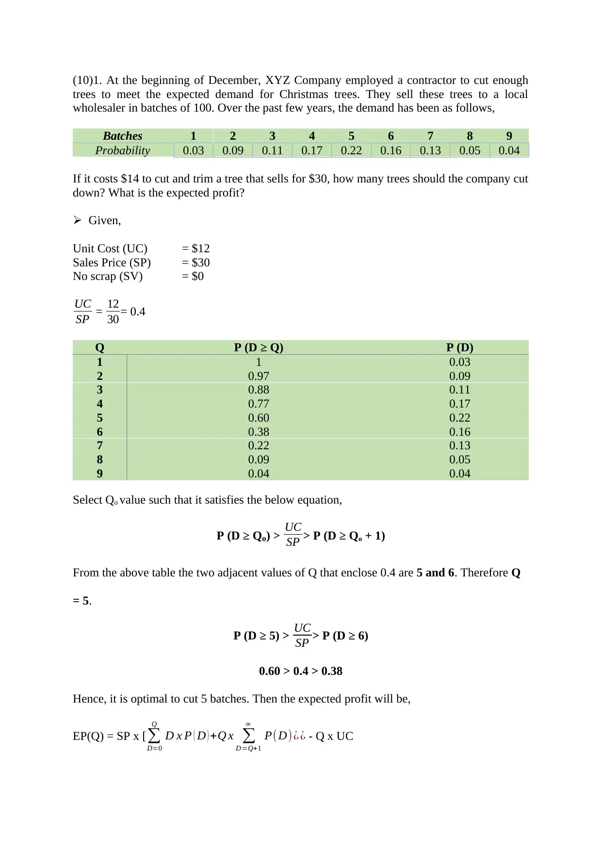
Batches 1 2 3 4 5 6 7 8 9
Probability 0.03 0.09 0.11 0.17 0.22 0.16 0.13 0.05 0.04
If it costs $14 to cut and trim a tree that sells for $30, how many trees should the company cut
down? What is the expected profit?
 Given,
Unit Cost (UC) = $12
Sales Price (SP) = $30
No scrap (SV) = $0
UC
SP = 12
30 = 0.4
Q P (D ≥ Q) P (D)
1 1 0.03
2 0.97 0.09
3 0.88 0.11
4 0.77 0.17
5 0.60 0.22
6 0.38 0.16
7 0.22 0.13
8 0.09 0.05
9 0.04 0.04
Select Qo value such that it satisfies the below equation,
P (D ≥ Qo) > UC
SP > P (D ≥ Qo + 1)
From the above table the two adjacent values of Q that enclose 0.4 are 5 and 6. Therefore Q
= 5.
P (D ≥ 5) > UC
SP > P (D ≥ 6)
0.60 > 0.4 > 0.38
Hence, it is optimal to cut 5 batches. Then the expected profit will be,
EP(Q) = SP x [∑
D=0
Q
D x P ( D ) +Q x ∑
D =Q+1
∞
P(D)¿ ¿ - Q x UC

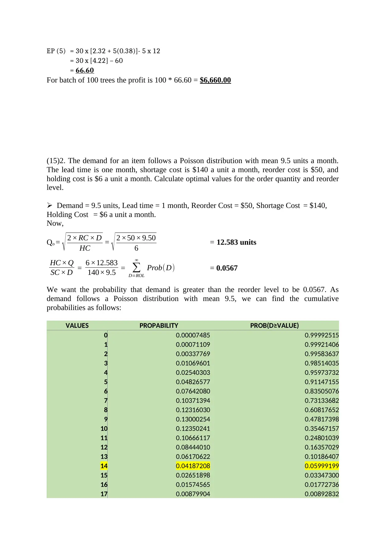
EP (5) = 30 x [2.32 + 5(0.38)]- 5 x 12
= 30 x [4.22] – 60
= 66.60
For batch of 100 trees the profit is 100 * 66.60 = $6,660.00
(15)2. The demand for an item follows a Poisson distribution with mean 9.5 units a month.
The lead time is one month, shortage cost is $140 a unit a month, reorder cost is $50, and
holding cost is $6 a unit a month. Calculate optimal values for the order quantity and reorder
level.
 Demand = 9.5 units, Lead time = 1 month, Reorder Cost = $50, Shortage Cost = $140,
Holding Cost = $6 a unit a month.
Now,
Qo = √ 2 × RC × D
HC = √ 2 ×50 × 9.50
6 = 12.583 units
HC × Q
SC × D = 6 ×12.583
140× 9.5 = ∑
D=ROL
∞
Prob(D) = 0.0567
We want the probability that demand is greater than the reorder level to be 0.0567. As
demand follows a Poisson distribution with mean 9.5, we can find the cumulative
probabilities as follows:
VALUES PROPABILITY PROB(D≥VALUE)
0 0.00007485 0.99992515
1 0.00071109 0.99921406
2 0.00337769 0.99583637
3 0.01069601 0.98514035
4 0.02540303 0.95973732
5 0.04826577 0.91147155
6 0.07642080 0.83505076
7 0.10371394 0.73133682
8 0.12316030 0.60817652
9 0.13000254 0.47817398
10 0.12350241 0.35467157
11 0.10666117 0.24801039
12 0.08444010 0.16357029
13 0.06170622 0.10186407
14 0.04187208 0.05999199
15 0.02651898 0.03347300
16 0.01574565 0.01772736
17 0.00879904 0.00892832

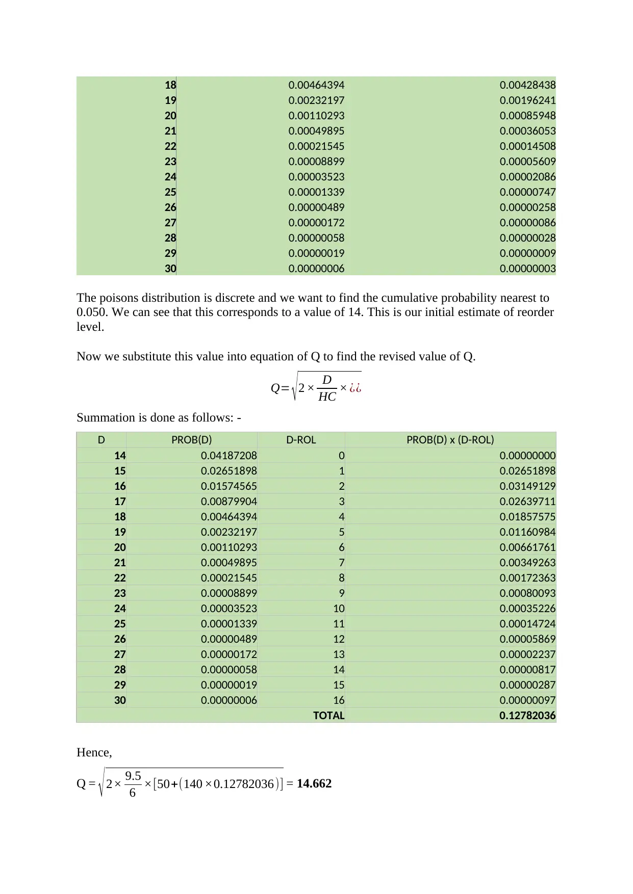
18 0.00464394 0.00428438
19 0.00232197 0.00196241
20 0.00110293 0.00085948
21 0.00049895 0.00036053
22 0.00021545 0.00014508
23 0.00008899 0.00005609
24 0.00003523 0.00002086
25 0.00001339 0.00000747
26 0.00000489 0.00000258
27 0.00000172 0.00000086
28 0.00000058 0.00000028
29 0.00000019 0.00000009
30 0.00000006 0.00000003
The poisons distribution is discrete and we want to find the cumulative probability nearest to
0.050. We can see that this corresponds to a value of 14. This is our initial estimate of reorder
level.
Now we substitute this value into equation of Q to find the revised value of Q.
Q= √ 2 × D
HC × ¿¿
Summation is done as follows: -
D PROB(D) D-ROL PROB(D) x (D-ROL)
14 0.04187208 0 0.00000000
15 0.02651898 1 0.02651898
16 0.01574565 2 0.03149129
17 0.00879904 3 0.02639711
18 0.00464394 4 0.01857575
19 0.00232197 5 0.01160984
20 0.00110293 6 0.00661761
21 0.00049895 7 0.00349263
22 0.00021545 8 0.00172363
23 0.00008899 9 0.00080093
24 0.00003523 10 0.00035226
25 0.00001339 11 0.00014724
26 0.00000489 12 0.00005869
27 0.00000172 13 0.00002237
28 0.00000058 14 0.00000817
29 0.00000019 15 0.00000287
30 0.00000006 16 0.00000097
TOTAL 0.12782036
Hence,
Q = √2× 9.5
6 ×[50+(140 ×0.12782036)] = 14.662

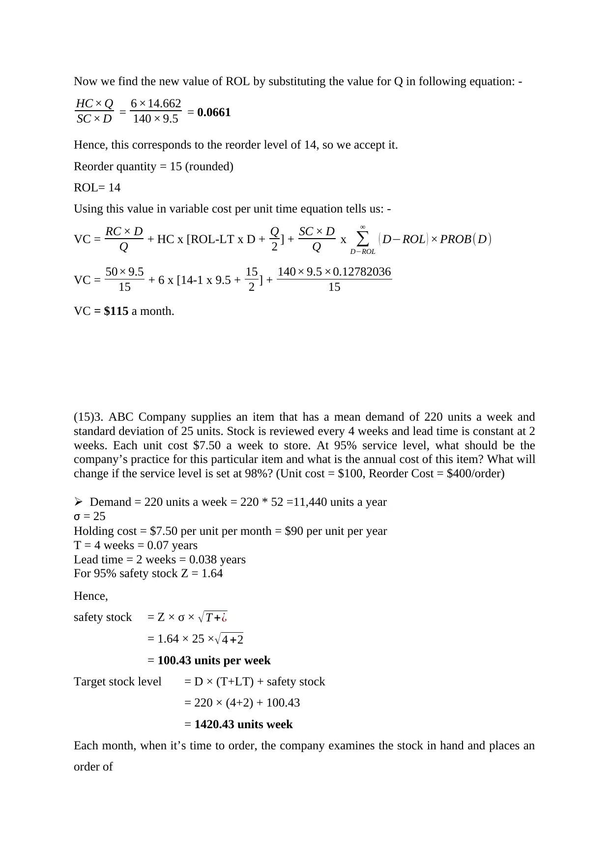
Now we find the new value of ROL by substituting the value for Q in following equation: -
HC × Q
SC × D = 6 ×14.662
140 × 9.5 = 0.0661
Hence, this corresponds to the reorder level of 14, so we accept it.
Reorder quantity = 15 (rounded)
ROL= 14
Using this value in variable cost per unit time equation tells us: -
VC = RC × D
Q + HC x [ROL-LT x D + Q
2 ] + SC × D
Q x ∑
D−ROL
∞
( D−ROL ) × PROB( D)
VC = 50× 9.5
15 + 6 x [14-1 x 9.5 + 15
2 ] + 140× 9.5 ×0.12782036
15
VC = $115 a month.
(15)3. ABC Company supplies an item that has a mean demand of 220 units a week and
standard deviation of 25 units. Stock is reviewed every 4 weeks and lead time is constant at 2
weeks. Each unit cost $7.50 a week to store. At 95% service level, what should be the
company’s practice for this particular item and what is the annual cost of this item? What will
change if the service level is set at 98%? (Unit cost = $100, Reorder Cost = $400/order)
 Demand = 220 units a week = 220 * 52 =11,440 units a year
σ = 25
Holding cost = $7.50 per unit per month = $90 per unit per year
T = 4 weeks = 0.07 years
Lead time = 2 weeks = 0.038 years
For 95% safety stock Z = 1.64
Hence,
safety stock = Z × σ × √T +¿
= 1.64 × 25 ×√4 +2
= 100.43 units per week
Target stock level = D × (T+LT) + safety stock
= 220 × (4+2) + 100.43
= 1420.43 units week
Each month, when it’s time to order, the company examines the stock in hand and places an
order of

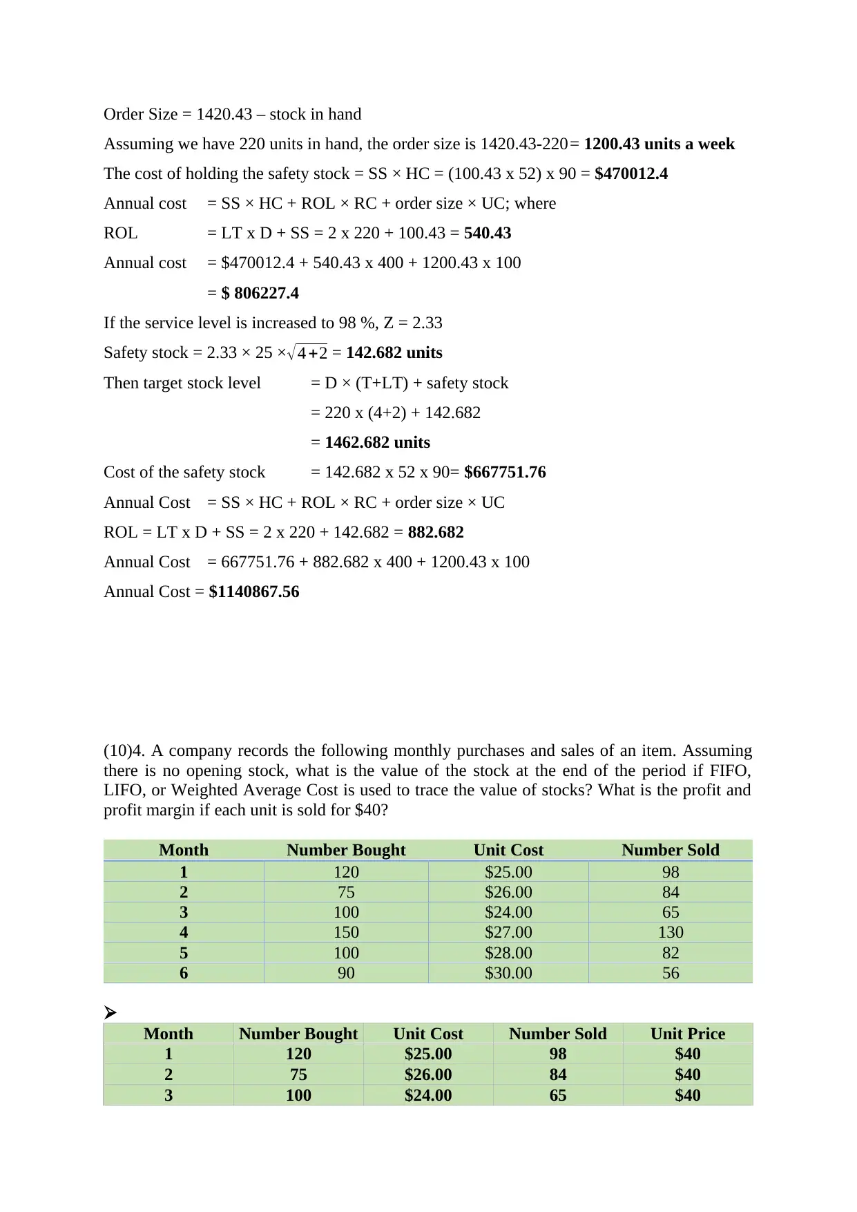
Order Size = 1420.43 – stock in hand
Assuming we have 220 units in hand, the order size is 1420.43-220= 1200.43 units a week
The cost of holding the safety stock = SS × HC = (100.43 x 52) x 90 = $470012.4
Annual cost = SS × HC + ROL × RC + order size × UC; where
ROL = LT x D + SS = 2 x 220 + 100.43 = 540.43
Annual cost = $470012.4 + 540.43 x 400 + 1200.43 x 100
= $ 806227.4
If the service level is increased to 98 %, Z = 2.33
Safety stock = 2.33 × 25 ×√4 +2 = 142.682 units
Then target stock level = D × (T+LT) + safety stock
= 220 x (4+2) + 142.682
= 1462.682 units
Cost of the safety stock = 142.682 x 52 x 90= $667751.76
Annual Cost = SS × HC + ROL × RC + order size × UC
ROL = LT x D + SS = 2 x 220 + 142.682 = 882.682
Annual Cost = 667751.76 + 882.682 x 400 + 1200.43 x 100
Annual Cost = $1140867.56
(10)4. A company records the following monthly purchases and sales of an item. Assuming
there is no opening stock, what is the value of the stock at the end of the period if FIFO,
LIFO, or Weighted Average Cost is used to trace the value of stocks? What is the profit and
profit margin if each unit is sold for $40?
Month Number Bought Unit Cost Number Sold
1 120 $25.00 98
2 75 $26.00 84
3 100 $24.00 65
4 150 $27.00 130
5 100 $28.00 82
6 90 $30.00 56

Month Number Bought Unit Cost Number Sold Unit Price
1 120 $25.00 98 $40
2 75 $26.00 84 $40
3 100 $24.00 65 $40

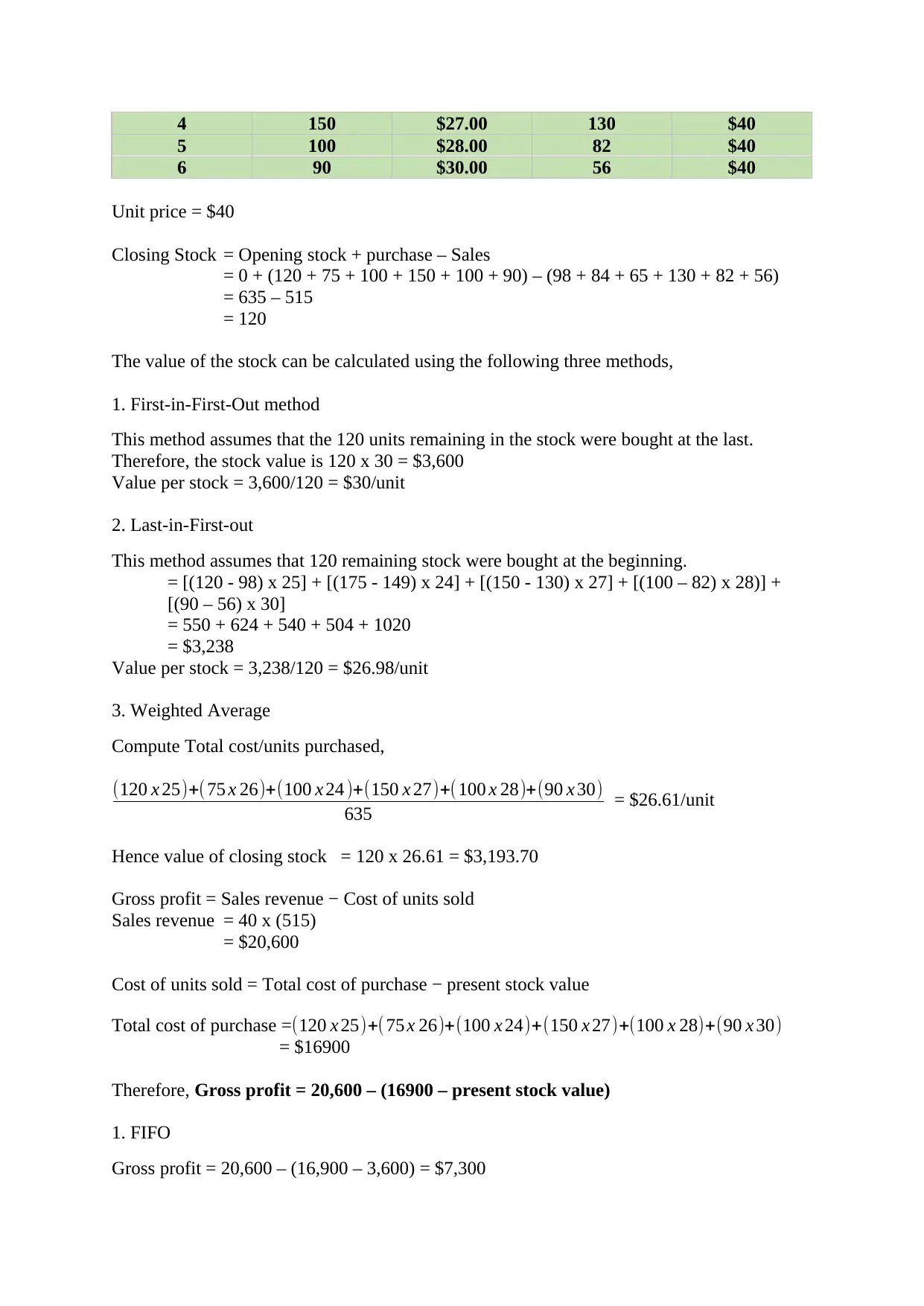
4 150 $27.00 130 $40
5 100 $28.00 82 $40
6 90 $30.00 56 $40
Unit price = $40
Closing Stock = Opening stock + purchase – Sales
= 0 + (120 + 75 + 100 + 150 + 100 + 90) – (98 + 84 + 65 + 130 + 82 + 56)
= 635 – 515
= 120
The value of the stock can be calculated using the following three methods,
1. First-in-First-Out method
This method assumes that the 120 units remaining in the stock were bought at the last.
Therefore, the stock value is 120 x 30 = $3,600
Value per stock = 3,600/120 = $30/unit
2. Last-in-First-out
This method assumes that 120 remaining stock were bought at the beginning.
= [(120 - 98) x 25] + [(175 - 149) x 24] + [(150 - 130) x 27] + [(100 – 82) x 28)] +
[(90 – 56) x 30]
= 550 + 624 + 540 + 504 + 1020
= $3,238
Value per stock = 3,238/120 = $26.98/unit
3. Weighted Average
Compute Total cost/units purchased,
(120 x 25)+( 75 x 26)+(100 x 24 )+(150 x 27)+( 100 x 28)+(90 x 30)
635 = $26.61/unit
Hence value of closing stock = 120 x 26.61 = $3,193.70
Gross profit = Sales revenue − Cost of units sold
Sales revenue = 40 x (515)
= $20,600
Cost of units sold = Total cost of purchase − present stock value
Total cost of purchase =(120 x 25)+( 75 x 26)+(100 x 24)+(150 x 27)+(100 x 28)+(90 x 30)
= $16900
Therefore, Gross profit = 20,600 – (16900 – present stock value)
1. FIFO
Gross profit = 20,600 – (16,900 – 3,600) = $7,300

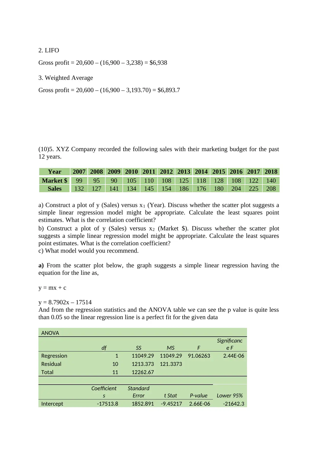
2. LIFO
Gross profit = 20,600 – (16,900 – 3,238) = $6,938
3. Weighted Average
Gross profit = 20,600 – (16,900 – 3,193.70) = $6,893.7
(10)5. XYZ Company recorded the following sales with their marketing budget for the past
12 years.
Year 2007 2008 2009 2010 2011 2012 2013 2014 2015 2016 2017 2018
Market $ 99 95 90 105 110 108 125 118 128 108 122 140
Sales 132 127 141 134 145 154 186 176 180 204 225 208
a) Construct a plot of y (Sales) versus x1 (Year). Discuss whether the scatter plot suggests a
simple linear regression model might be appropriate. Calculate the least squares point
estimates. What is the correlation coefficient?
b) Construct a plot of y (Sales) versus x2 (Market $). Discuss whether the scatter plot
suggests a simple linear regression model might be appropriate. Calculate the least squares
point estimates. What is the correlation coefficient?
c) What model would you recommend.
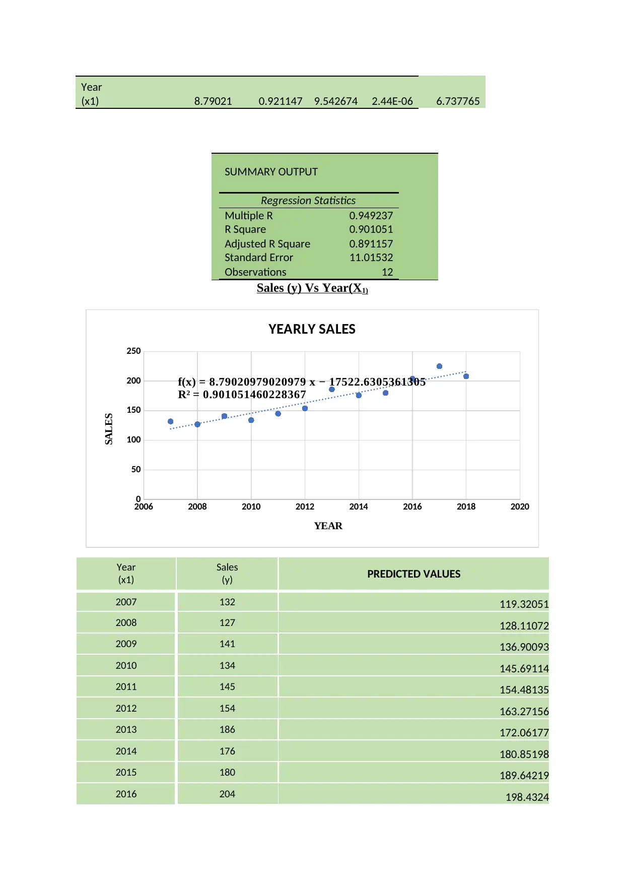
a) From the scatter plot below, the graph suggests a simple linear regression having the
equation for the line as,
y = mx + c
y = 8.7902x – 17514
And from the regression statistics and the ANOVA table we can see the p value is quite less
than 0.05 so the linear regression line is a perfect fit for the given data
ANOVA
df SS MS F
Significanc
e F
Regression 1 11049.29 11049.29 91.06263 2.44E-06
Residual 10 1213.373 121.3373
Total 11 12262.67
Coefficient
s
Standard
Error t Stat P-value Lower 95%
Intercept -17513.8 1852.891 -9.45217 2.66E-06 -21642.3

Year
(x1) 8.79021 0.921147 9.542674 2.44E-06 6.737765
SUMMARY OUTPUT
Regression Statistics
Multiple R 0.949237
R Square 0.901051
Adjusted R Square 0.891157
Standard Error 11.01532
Observations 12
Sales (y) Vs Year(X1)
2006 2008 2010 2012 2014 2016 2018 2020
0
50
100
150
200
250
f(x) = 8.79020979020979 x − 17522.6305361305
R² = 0.901051460228367
YEARLY SALES
YEAR
SALES
Year
(x1)
Sales
(y) PREDICTED VALUES
2007 132 119.32051
2008 127 128.11072
2009 141 136.90093
2010 134 145.69114
2011 145 154.48135
2012 154 163.27156
2013 186 172.06177
2014 176 180.85198
2015 180 189.64219
2016 204 198.4324

2017 225 207.22261
2018 208 216.01282
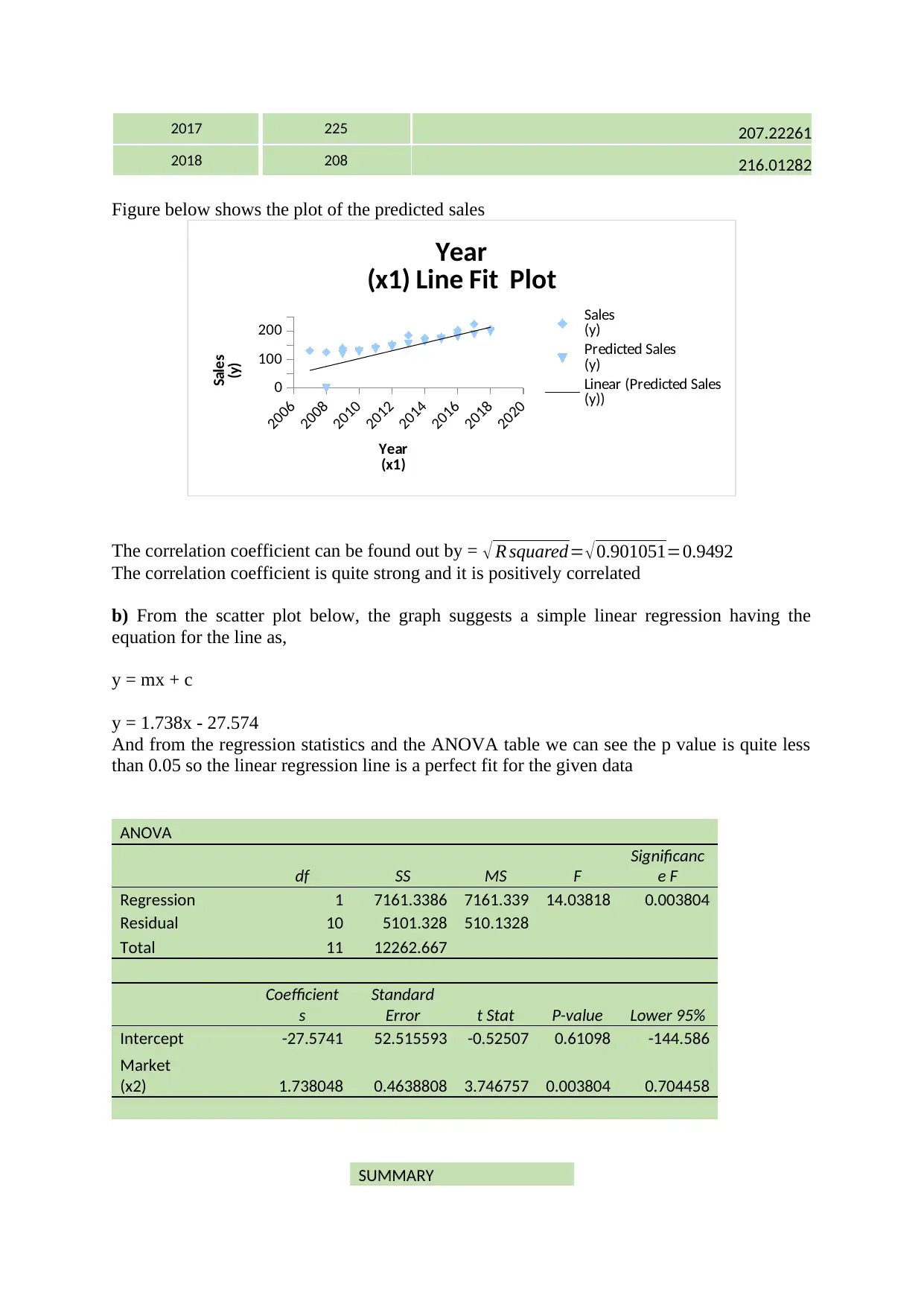
Figure below shows the plot of the predicted sales
2006
2008
2010
2012
2014
2016
2018
2020
0
100
200
Year
(x1) Line Fit Plot
Sales
(y)
Predicted Sales
(y)
Linear (Predicted Sales
(y))
Year
(x1)
Sales
(y)
The correlation coefficient can be found out by = √ R squared= √ 0.901051=0.9492
The correlation coefficient is quite strong and it is positively correlated
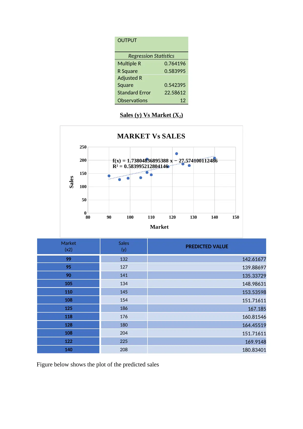
b) From the scatter plot below, the graph suggests a simple linear regression having the
equation for the line as,
y = mx + c
y = 1.738x - 27.574
And from the regression statistics and the ANOVA table we can see the p value is quite less
than 0.05 so the linear regression line is a perfect fit for the given data
ANOVA
df SS MS F
Significanc
e F
Regression 1 7161.3386 7161.339 14.03818 0.003804
Residual 10 5101.328 510.1328
Total 11 12262.667
Coefficient
s
Standard
Error t Stat P-value Lower 95%
Intercept -27.5741 52.515593 -0.52507 0.61098 -144.586
Market
(x2) 1.738048 0.4638808 3.746757 0.003804 0.704458
SUMMARY

OUTPUT
Regression Statistics
Multiple R 0.764196
R Square 0.583995
Adjusted R
Square 0.542395
Standard Error 22.58612
Observations 12
Sales (y) Vs Market (X2)
80 90 100 110 120 130 140 150
0
50
100
150
200
250
f(x) = 1.73804836895388 x − 27.574100112486
R² = 0.583995212804146
MARKET Vs SALES
Market
Sales
Market
(x2)
Sales
(y) PREDICTED VALUE
99 132 142.61677
95 127 139.88697
90 141 135.33729
105 134 148.98631
110 145 153.53598
108 154 151.71611
125 186 167.185
118 176 160.81546
128 180 164.45519
108 204 151.71611
122 225 169.9148
140 208 180.83401
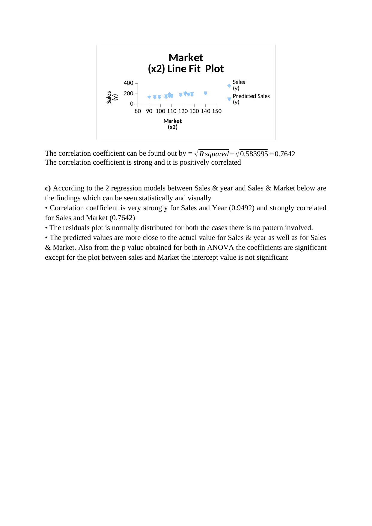
Figure below shows the plot of the predicted sales

80 90 100 110 120 130 140 150
0
200
400
Market
(x2) Line Fit Plot
Sales
(y)
Predicted Sales
(y)
Market
(x2)
Sales
(y)
The correlation coefficient can be found out by = √ R squared= √0.583995=0.7642
The correlation coefficient is strong and it is positively correlated
c) According to the 2 regression models between Sales & year and Sales & Market below are
the findings which can be seen statistically and visually
• Correlation coefficient is very strongly for Sales and Year (0.9492) and strongly correlated
for Sales and Market (0.7642)
• The residuals plot is normally distributed for both the cases there is no pattern involved.
• The predicted values are more close to the actual value for Sales & year as well as for Sales
& Market. Also from the p value obtained for both in ANOVA the coefficients are significant
except for the plot between sales and Market the intercept value is not significant