401076 Introduction to Epidemiology

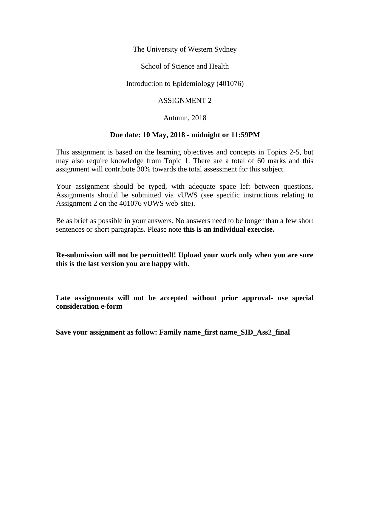
The University of Western Sydney
School of Science and Health
Introduction to Epidemiology (401076)
ASSIGNMENT 2
Autumn, 2018
Due date: 10 May, 2018 - midnight or 11:59PM
This assignment is based on the learning objectives and concepts in Topics 2-5, but
may also require knowledge from Topic 1. There are a total of 60 marks and this
assignment will contribute 30% towards the total assessment for this subject.
Your assignment should be typed, with adequate space left between questions.
Assignments should be submitted via vUWS (see specific instructions relating to
Assignment 2 on the 401076 vUWS web-site).
Be as brief as possible in your answers. No answers need to be longer than a few short
sentences or short paragraphs. Please note this is an individual exercise.
Re-submission will not be permitted!! Upload your work only when you are sure
this is the last version you are happy with.
Late assignments will not be accepted without prior approval- use special
consideration e-form
Save your assignment as follow: Family name_first name_SID_Ass2_final

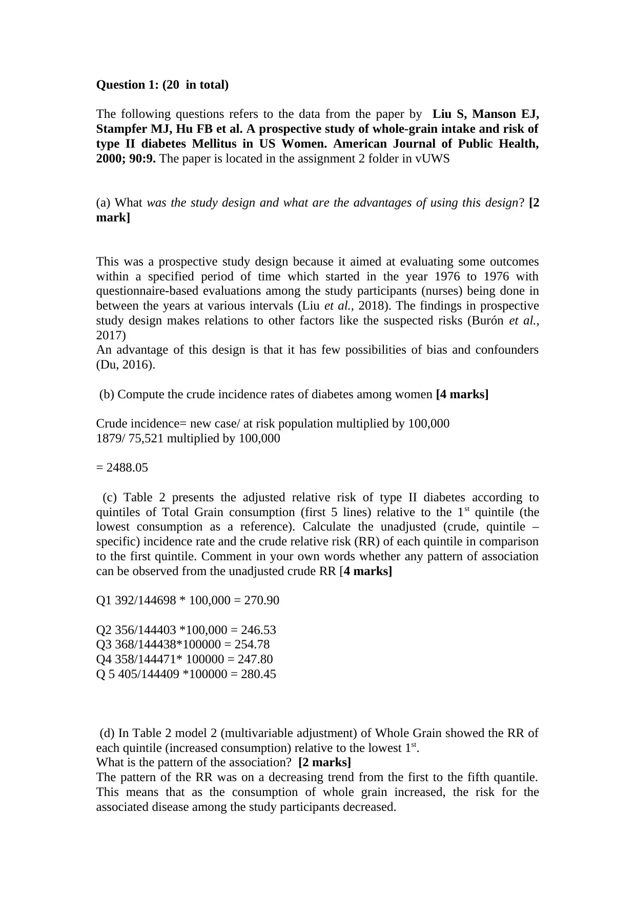
Question 1: (20 in total)
The following questions refers to the data from the paper by Liu S, Manson EJ,
Stampfer MJ, Hu FB et al. A prospective study of whole-grain intake and risk of
type II diabetes Mellitus in US Women. American Journal of Public Health,
2000; 90:9. The paper is located in the assignment 2 folder in vUWS
(a) What was the study design and what are the advantages of using this design? [2
mark]
This was a prospective study design because it aimed at evaluating some outcomes
within a specified period of time which started in the year 1976 to 1976 with
questionnaire-based evaluations among the study participants (nurses) being done in
between the years at various intervals (Liu et al., 2018). The findings in prospective
study design makes relations to other factors like the suspected risks (Burón et al.,
2017)
An advantage of this design is that it has few possibilities of bias and confounders
(Du, 2016).
(b) Compute the crude incidence rates of diabetes among women [4 marks]
Crude incidence= new case/ at risk population multiplied by 100,000
1879/ 75,521 multiplied by 100,000
= 2488.05
(c) Table 2 presents the adjusted relative risk of type II diabetes according to
quintiles of Total Grain consumption (first 5 lines) relative to the 1st quintile (the
lowest consumption as a reference). Calculate the unadjusted (crude, quintile –
specific) incidence rate and the crude relative risk (RR) of each quintile in comparison
to the first quintile. Comment in your own words whether any pattern of association
can be observed from the unadjusted crude RR [4 marks]
Q1 392/144698 * 100,000 = 270.90
Q2 356/144403 *100,000 = 246.53
Q3 368/144438*100000 = 254.78
Q4 358/144471* 100000 = 247.80
Q 5 405/144409 *100000 = 280.45
(d) In Table 2 model 2 (multivariable adjustment) of Whole Grain showed the RR of
each quintile (increased consumption) relative to the lowest 1st.
What is the pattern of the association? [2 marks]
The pattern of the RR was on a decreasing trend from the first to the fifth quantile.
This means that as the consumption of whole grain increased, the risk for the
associated disease among the study participants decreased.

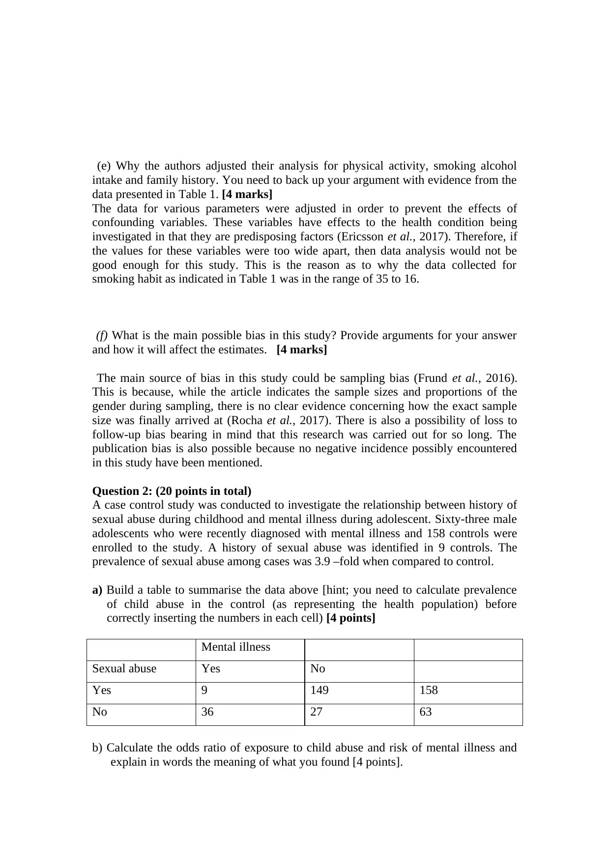
(e) Why the authors adjusted their analysis for physical activity, smoking alcohol
intake and family history. You need to back up your argument with evidence from the
data presented in Table 1. [4 marks]
The data for various parameters were adjusted in order to prevent the effects of
confounding variables. These variables have effects to the health condition being
investigated in that they are predisposing factors (Ericsson et al., 2017). Therefore, if
the values for these variables were too wide apart, then data analysis would not be
good enough for this study. This is the reason as to why the data collected for
smoking habit as indicated in Table 1 was in the range of 35 to 16.
(f) What is the main possible bias in this study? Provide arguments for your answer
and how it will affect the estimates. [4 marks]
The main source of bias in this study could be sampling bias (Frund et al., 2016).
This is because, while the article indicates the sample sizes and proportions of the
gender during sampling, there is no clear evidence concerning how the exact sample
size was finally arrived at (Rocha et al., 2017). There is also a possibility of loss to
follow-up bias bearing in mind that this research was carried out for so long. The
publication bias is also possible because no negative incidence possibly encountered
in this study have been mentioned.
Question 2: (20 points in total)
A case control study was conducted to investigate the relationship between history of
sexual abuse during childhood and mental illness during adolescent. Sixty-three male
adolescents who were recently diagnosed with mental illness and 158 controls were
enrolled to the study. A history of sexual abuse was identified in 9 controls. The
prevalence of sexual abuse among cases was 3.9 –fold when compared to control.
a) Build a table to summarise the data above [hint; you need to calculate prevalence
of child abuse in the control (as representing the health population) before
correctly inserting the numbers in each cell) [4 points]
Mental illness
Sexual abuse Yes No
Yes 9 149 158
No 36 27 63
b) Calculate the odds ratio of exposure to child abuse and risk of mental illness and
explain in words the meaning of what you found [4 points].

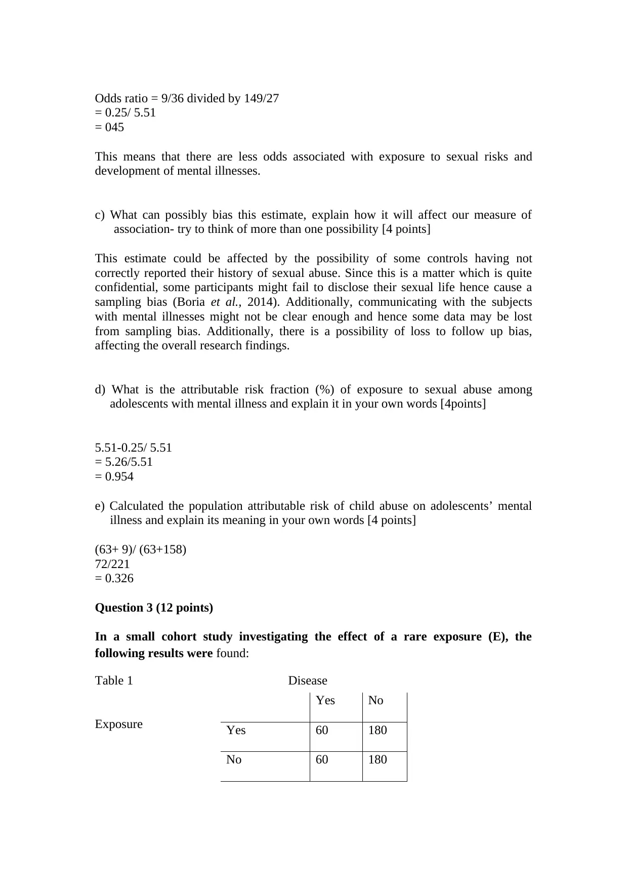
Odds ratio = 9/36 divided by 149/27
= 0.25/ 5.51
= 045
This means that there are less odds associated with exposure to sexual risks and
development of mental illnesses.
c) What can possibly bias this estimate, explain how it will affect our measure of
association- try to think of more than one possibility [4 points]
This estimate could be affected by the possibility of some controls having not
correctly reported their history of sexual abuse. Since this is a matter which is quite
confidential, some participants might fail to disclose their sexual life hence cause a
sampling bias (Boria et al., 2014). Additionally, communicating with the subjects
with mental illnesses might not be clear enough and hence some data may be lost
from sampling bias. Additionally, there is a possibility of loss to follow up bias,
affecting the overall research findings.
d) What is the attributable risk fraction (%) of exposure to sexual abuse among
adolescents with mental illness and explain it in your own words [4points]
5.51-0.25/ 5.51
= 5.26/5.51
= 0.954
e) Calculated the population attributable risk of child abuse on adolescents’ mental
illness and explain its meaning in your own words [4 points]
(63+ 9)/ (63+158)
72/221
= 0.326
Question 3 (12 points)
In a small cohort study investigating the effect of a rare exposure (E), the
following results were found:
Table 1 Disease
Exposure
Yes No
Yes 60 180
No 60 180

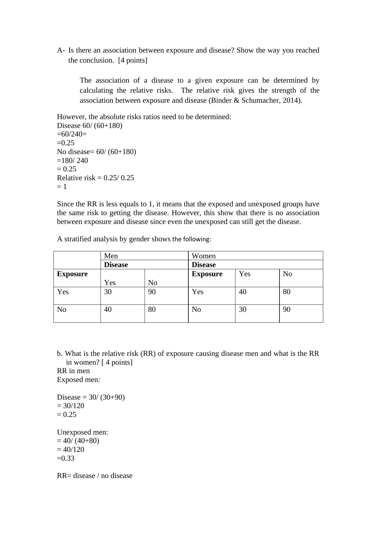
A- Is there an association between exposure and disease? Show the way you reached
the conclusion. [4 points]
The association of a disease to a given exposure can be determined by
calculating the relative risks. The relative risk gives the strength of the
association between exposure and disease (Binder & Schumacher, 2014).
However, the absolute risks ratios need to be determined:
Disease 60/ (60+180)
=60/240=
=0.25
No disease= 60/ (60+180)
=180/ 240
= 0.25
Relative risk = 0.25/ 0.25
= 1
Since the RR is less equals to 1, it means that the exposed and unexposed groups have
the same risk to getting the disease. However, this show that there is no association
between exposure and disease since even the unexposed can still get the disease.
A stratified analysis by gender shows the following:
Men Women
Disease Disease
Exposure
Yes No
Exposure Yes No
Yes 30 90 Yes 40 80
No 40 80 No 30 90
b. What is the relative risk (RR) of exposure causing disease men and what is the RR
in women? [ 4 points]
RR in men
Exposed men:
Disease = 30/ (30+90)
= 30/120
= 0.25
Unexposed men:
= 40/ (40+80)
= 40/120
=0.33
RR= disease / no disease

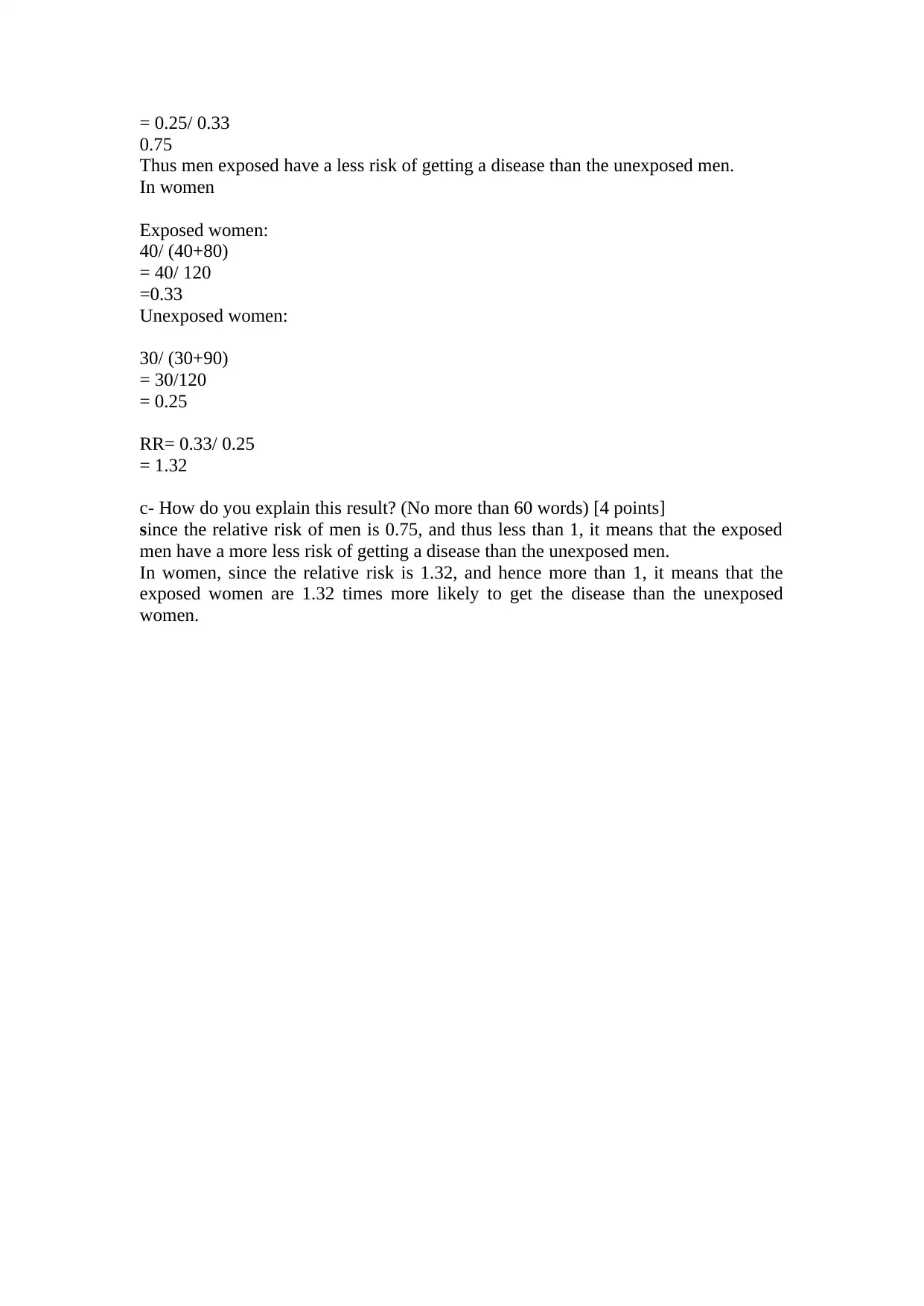
= 0.25/ 0.33
0.75
Thus men exposed have a less risk of getting a disease than the unexposed men.
In women
Exposed women:
40/ (40+80)
= 40/ 120
=0.33
Unexposed women:
30/ (30+90)
= 30/120
= 0.25
RR= 0.33/ 0.25
= 1.32
c- How do you explain this result? (No more than 60 words) [4 points]
since the relative risk of men is 0.75, and thus less than 1, it means that the exposed
men have a more less risk of getting a disease than the unexposed men.
In women, since the relative risk is 1.32, and hence more than 1, it means that the
exposed women are 1.32 times more likely to get the disease than the unexposed
women.

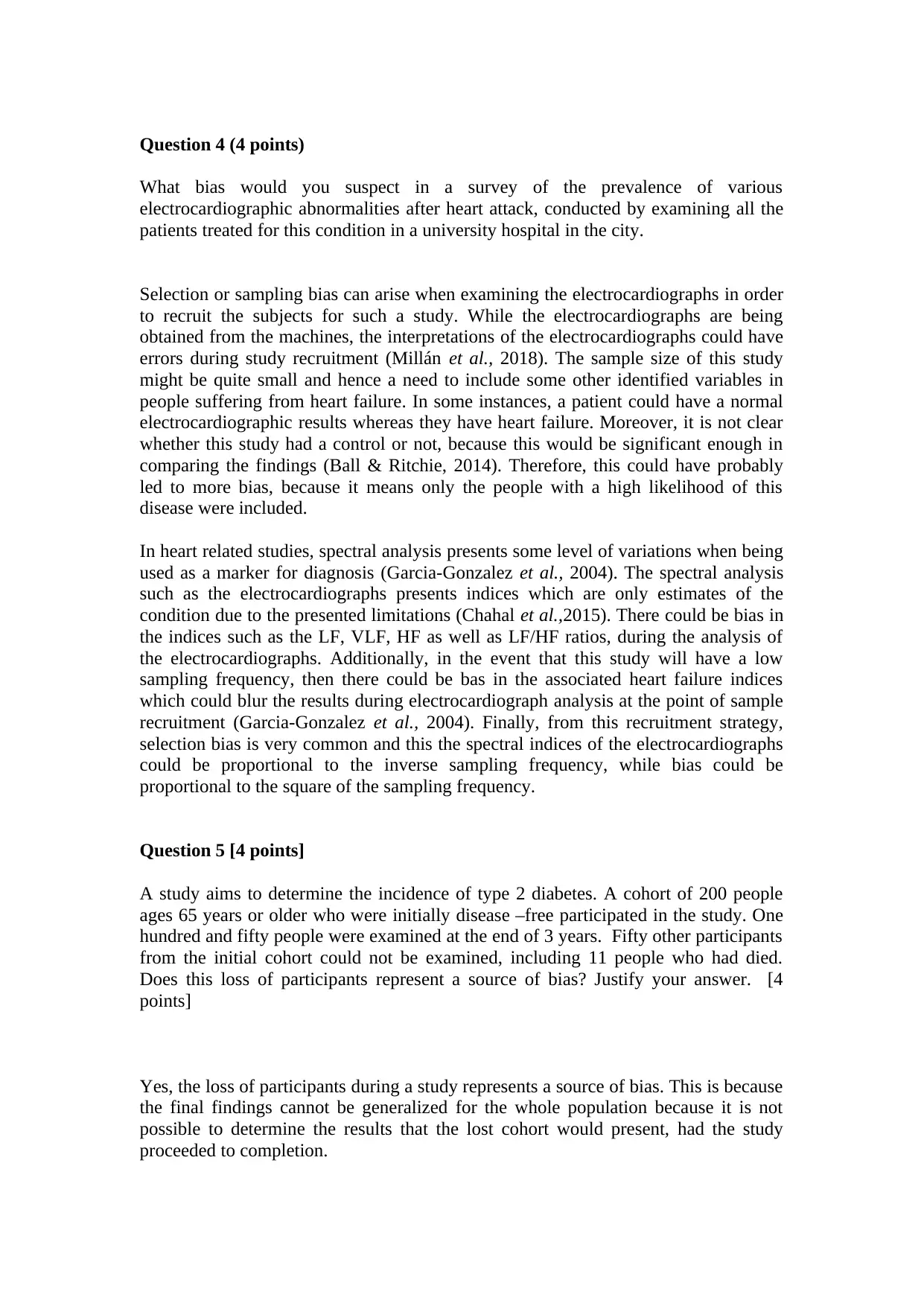
Question 4 (4 points)
What bias would you suspect in a survey of the prevalence of various
electrocardiographic abnormalities after heart attack, conducted by examining all the
patients treated for this condition in a university hospital in the city.
Selection or sampling bias can arise when examining the electrocardiographs in order
to recruit the subjects for such a study. While the electrocardiographs are being
obtained from the machines, the interpretations of the electrocardiographs could have
errors during study recruitment (Millán et al., 2018). The sample size of this study
might be quite small and hence a need to include some other identified variables in
people suffering from heart failure. In some instances, a patient could have a normal
electrocardiographic results whereas they have heart failure. Moreover, it is not clear
whether this study had a control or not, because this would be significant enough in
comparing the findings (Ball & Ritchie, 2014). Therefore, this could have probably
led to more bias, because it means only the people with a high likelihood of this
disease were included.
In heart related studies, spectral analysis presents some level of variations when being
used as a marker for diagnosis (Garcia-Gonzalez et al., 2004). The spectral analysis
such as the electrocardiographs presents indices which are only estimates of the
condition due to the presented limitations (Chahal et al.,2015). There could be bias in
the indices such as the LF, VLF, HF as well as LF/HF ratios, during the analysis of
the electrocardiographs. Additionally, in the event that this study will have a low
sampling frequency, then there could be bas in the associated heart failure indices
which could blur the results during electrocardiograph analysis at the point of sample
recruitment (Garcia-Gonzalez et al., 2004). Finally, from this recruitment strategy,
selection bias is very common and this the spectral indices of the electrocardiographs
could be proportional to the inverse sampling frequency, while bias could be
proportional to the square of the sampling frequency.
Question 5 [4 points]
A study aims to determine the incidence of type 2 diabetes. A cohort of 200 people
ages 65 years or older who were initially disease –free participated in the study. One
hundred and fifty people were examined at the end of 3 years. Fifty other participants
from the initial cohort could not be examined, including 11 people who had died.
Does this loss of participants represent a source of bias? Justify your answer. [4
points]
Yes, the loss of participants during a study represents a source of bias. This is because
the final findings cannot be generalized for the whole population because it is not
possible to determine the results that the lost cohort would present, had the study
proceeded to completion.

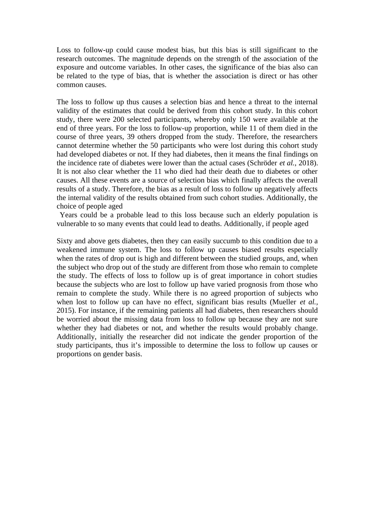
Loss to follow-up could cause modest bias, but this bias is still significant to the
research outcomes. The magnitude depends on the strength of the association of the
exposure and outcome variables. In other cases, the significance of the bias also can
be related to the type of bias, that is whether the association is direct or has other
common causes.
The loss to follow up thus causes a selection bias and hence a threat to the internal
validity of the estimates that could be derived from this cohort study. In this cohort
study, there were 200 selected participants, whereby only 150 were available at the
end of three years. For the loss to follow-up proportion, while 11 of them died in the
course of three years, 39 others dropped from the study. Therefore, the researchers
cannot determine whether the 50 participants who were lost during this cohort study
had developed diabetes or not. If they had diabetes, then it means the final findings on
the incidence rate of diabetes were lower than the actual cases (Schröder et al., 2018).
It is not also clear whether the 11 who died had their death due to diabetes or other
causes. All these events are a source of selection bias which finally affects the overall
results of a study. Therefore, the bias as a result of loss to follow up negatively affects
the internal validity of the results obtained from such cohort studies. Additionally, the
choice of people aged
Years could be a probable lead to this loss because such an elderly population is
vulnerable to so many events that could lead to deaths. Additionally, if people aged
Sixty and above gets diabetes, then they can easily succumb to this condition due to a
weakened immune system. The loss to follow up causes biased results especially
when the rates of drop out is high and different between the studied groups, and, when
the subject who drop out of the study are different from those who remain to complete
the study. The effects of loss to follow up is of great importance in cohort studies
because the subjects who are lost to follow up have varied prognosis from those who
remain to complete the study. While there is no agreed proportion of subjects who
when lost to follow up can have no effect, significant bias results (Mueller et al.,
2015). For instance, if the remaining patients all had diabetes, then researchers should
be worried about the missing data from loss to follow up because they are not sure
whether they had diabetes or not, and whether the results would probably change.
Additionally, initially the researcher did not indicate the gender proportion of the
study participants, thus it’s impossible to determine the loss to follow up causes or
proportions on gender basis.

References
Ball, T. S., & Ritchie, S. R. (2014). Sampling biases of the BG-sentinel trap with
respect to physiology, age, and body size of adult Aedes aegypti (Diptera:
Culicidae). Journal of medical entomology, 47(4), 649-656.
Binder, N., & Schumacher, M. (2014). Missing information caused by death leads to
bias in relative risk estimates. Journal of clinical epidemiology, 67(10), 1111-
1120.
Boria, R. A., Olson, L. E., Goodman, S. M., & Anderson, R. P. (2014). Spatial
filtering to reduce sampling bias can improve the performance of ecological
niche models. Ecological Modelling, 275, 73-77.
Burón Pust, A., Alison, R., Blanks, R., Pirie, K., Gaitskell, K., Barnes, I., ... & Million
Women Study Collaborators. (2017). Heterogeneity of colorectal cancer risk
by tumour characteristics: Large prospective study of UK women.
International journal of cancer, 140(5), 1082-1090.
Chahal, H., Bluemke, D. A., Wu, C. O., McClelland, R., Liu, K., Shea, S. J., ... &
Post, W. (2015). Heart failure risk prediction in the Multi-Ethnic Study of
Atherosclerosis. Heart, 101(1), 58-64.
Du, X., Pi, Y., Dreyer, R. P., Li, J., Li, X., Downing, N. S., ... & Guan, W. (2016).
The china patient‐centered evaluative assessment of cardiac events (PEACE)
prospective study of percutaneous coronary intervention: Study design.
Catheterization and Cardiovascular Interventions, 88(7), E212-E221.
Ericsson, N. R., Hendry, D. F., & Hood, S. B. (2017). Milton Friedman and Data
Adjustment (No. 2017-05-15). Board of Governors of the Federal Reserve
System (US).

Fründ, J., McCann, K. S., & Williams, N. M. (2016). Sampling bias is a challenge for
quantifying specialization and network structure: lessons from a quantitative
niche model. Oikos, 125(4), 502-513.
Garcia-Gonzalez, M. A., Fernandez-Chimeno, M., & Ramos-Castro, J. (2004). Bias
and uncertainty in heart rate variability spectral indices due to the finite ECG
sampling frequency. Physiological measurement, 25(2), 489.
Liu, S., Manson, J. E., Stampfer, M. J., Hu, F. B., Giovannucci, E., Colditz, G. A., ...
& Willett, W. C. (2000). A prospective study of whole-grain intake and risk of
type 2 diabetes mellitus in US women. American journal of public health,
90(9), 1409.
Millán, L. F., Livesey, N. J., Santee, M. L., & Clarmann, T. V. (2018). Characterizing
sampling and quality screening biases in infrared and microwave limb
sounding. Atmospheric Chemistry and Physics, 18(6), 4187-4199.
Mueller, N. T., Whyatt, R., Hoepner, L., Oberfield, S., Dominguez-Bello, M. G.,
Widen, E. M., ... & Rundle, A. (2015). Prenatal exposure to antibiotics,
cesarean section and risk of childhood obesity. International journal of
obesity, 39(4), 665.
Rocha, L. E., Thorson, A. E., Lambiotte, R., & Liljeros, F. (2017). Respondent‐driven
sampling bias induced by community structure and response rates in social
networks. Journal of the Royal Statistical Society: Series A (Statistics in
Society), 180(1), 99-118.
Schröder, M. L., Marlies, P., & Staartjes, V. E. (2018). Are patient-reported outcome
measures biased by method of follow-up? evaluating paper-based and digital
follow-up after lumbar fusion surgery. The Spine Journal.