Image Compression Project: Complex Wavelet Transform vs DWT Comparison

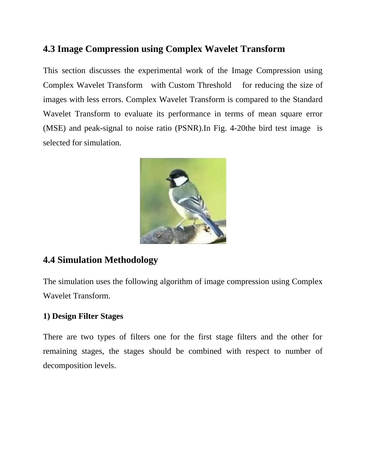
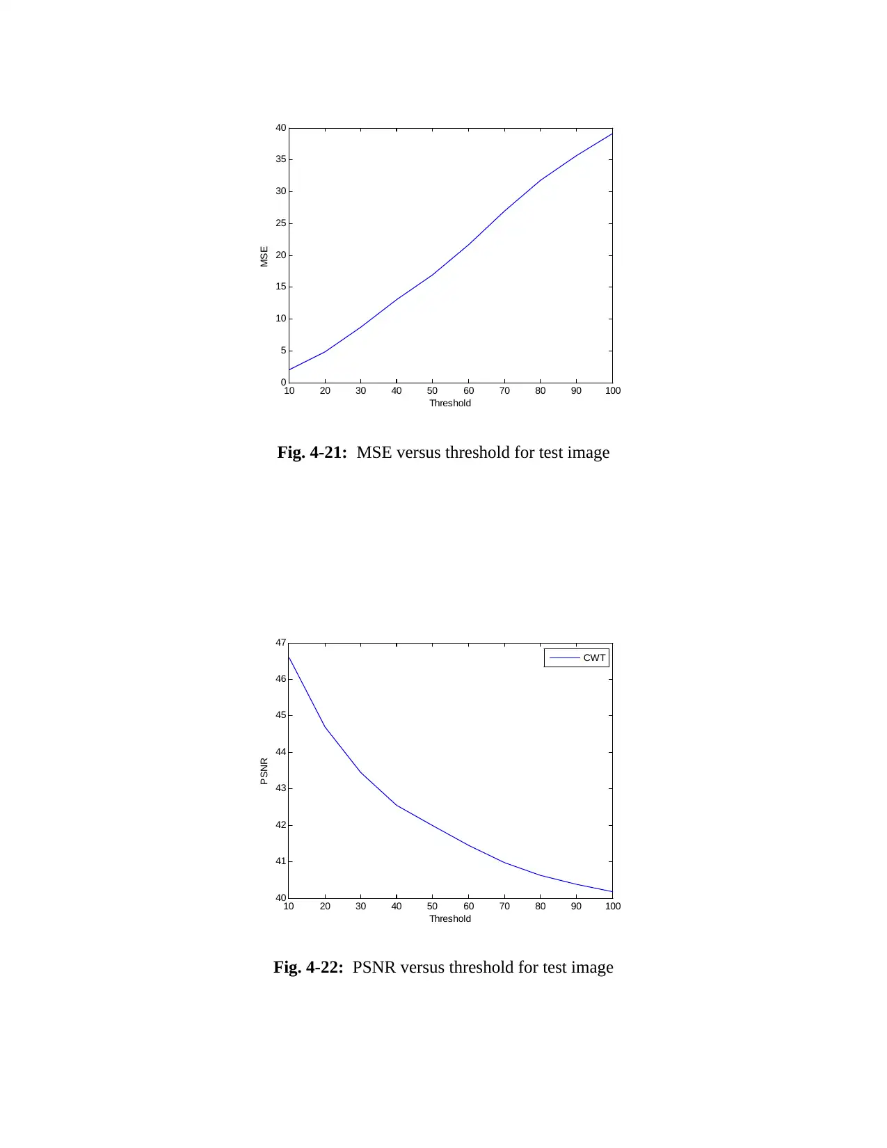
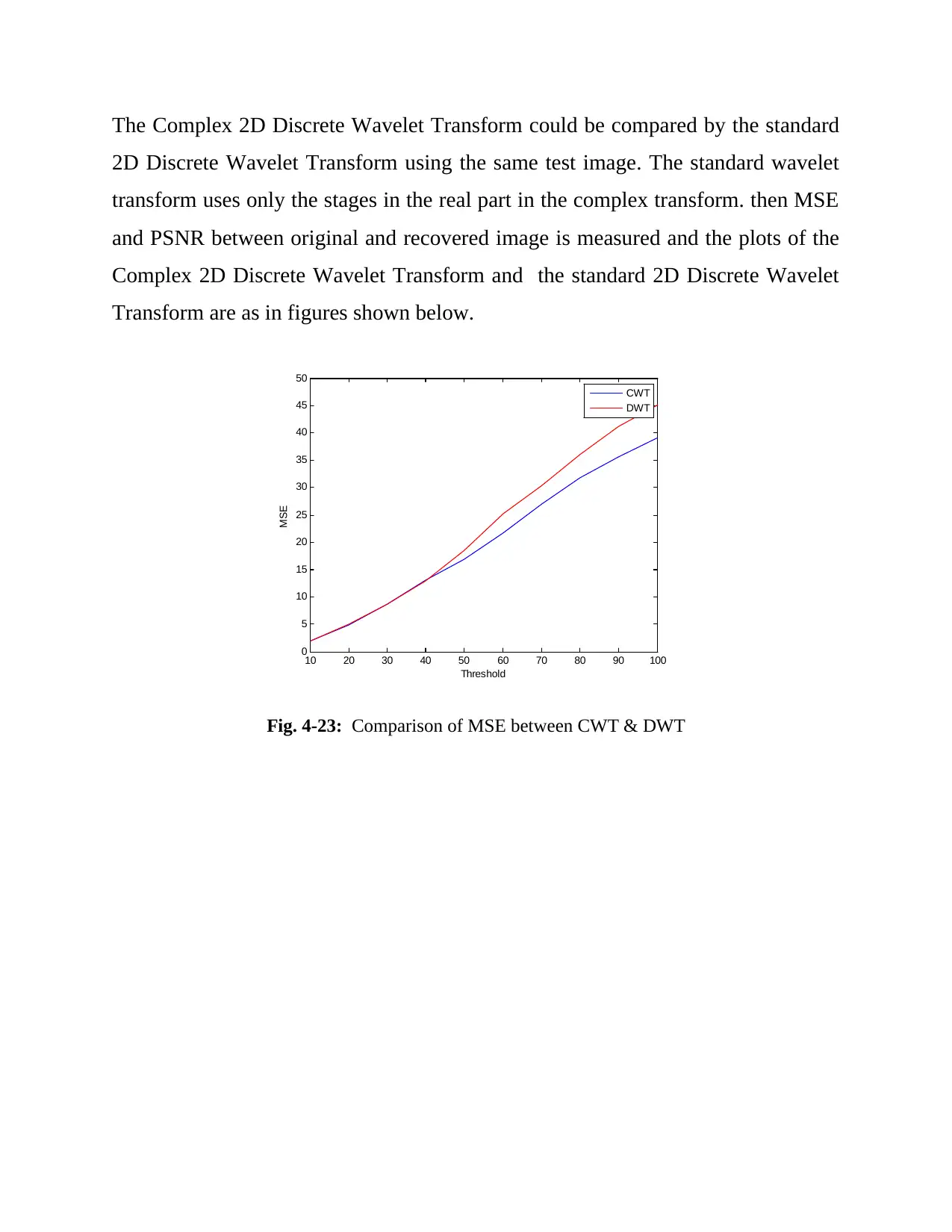
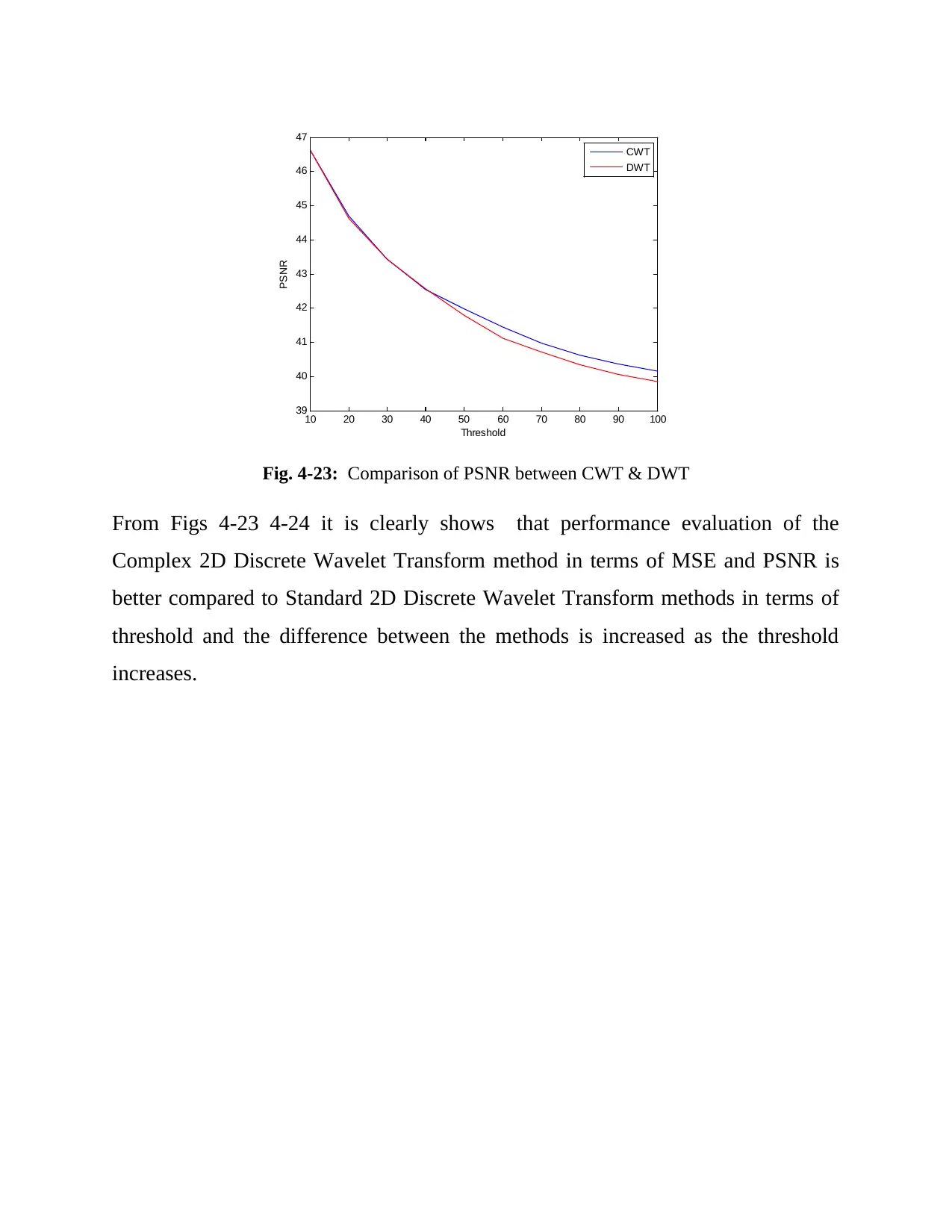
This project delves into image compression techniques, specifically focusing on the application of the Complex Wavelet Transform (CWT). The study outlines a simulation methodology that includes filter design, image resizing, and the separation of RGB components. It details the application of the complex 2D discrete wavelet transform, thresholding techniques (soft thresholding), and the inverse transform for image reconstruction. The project compares the performance of CWT with the standard 2D Discrete Wavelet Transform (DWT), evaluating their effectiveness using Mean Square Error (MSE) and Peak Signal-to-Noise Ratio (PSNR) metrics. The results, presented graphically, demonstrate the superior performance of CWT over DWT, especially with increasing threshold values, providing valuable insights into the efficiency of CWT in image compression applications.

4.3 Image Compression using Complex Wavelet Transform
This section discusses the experimental work of the Image Compression using
Complex Wavelet Transform with Custom Threshold for reducing the size of
images with less errors. Complex Wavelet Transform is compared to the Standard
Wavelet Transform to evaluate its performance in terms of mean square error
(MSE) and peak-signal to noise ratio (PSNR).In Fig. 4-20the bird test image is
selected for simulation.
4.4 Simulation Methodology
The simulation uses the following algorithm of image compression using Complex
Wavelet Transform.
1) Design Filter Stages
There are two types of filters one for the first stage filters and the other for
remaining stages, the stages should be combined with respect to number of
decomposition levels.

2) Reading the RGB image
the test image is read and resized to be 512×512×3. The Separation of Red, Green
and Blue components is applied in this algorithm.
3) Complex 2D Discrete Wavelet Transform
The complex 2-D dual-tree DWT also gives rise to wavelets in six distinct
directions, however, in this case there are two wavelets in each direction as will be
illustrated below. In each direction, one of the two wavelets can be interpreted as
the real part of a complex-valued 2D wavelet, while the other wavelet can be
interpreted as the imaginary part of a complex-valued 2D wavelet. The complex 2-
D dual-tree DWT of an image x is computed by the following function.
The wavelet coefficients w are stored as a cell array. For j = 1..J, p = 1..2, k = 1..2,
d = 1..3, w{j}{p}{k}{d} are the wavelet coefficients produced at scale j and
orientation (k,d). The dimension j represents the number of levels. With p = 1 we
get the real part, with p = 2 we get the imaginary part. The dimension d that the
operation is applied to the image RGB components.
If the image has N1 rows and N2 columns, then after applying the 1D analysis
filter bank to each column we have two subband images, each having N1/2 rows
and N2 columns; after applying the 1D analysis filter bank to each row of both of
the two subband images, we have four subband images, each having N1/2 rows
and N2/2 columns. In case of 3 level decomposition The 2D synthesis filter bank
combines the 3 subband images to obtain the original image of size N1 by N2.

4) Thresholding Technique
Thresholding is a technique used for image compression by setting some of its
pixels to zeros then the image file size is reduced. The proposed type of
thresholding is called Soft thresholding which deletes the coefficients under the
threshold, but scales the ones that are left. The general soft rule is defined by:
Where x is the image pixel λ is thresholdα is the parameter that controls the
shape of the thresholding function.
4) Inverse Complex 2D Discrete Wavelet Transform
The compressed image x is recovered from w using the inverse transform,
implemented by the similar technique that used in the wavelet transform but in
reverse order. The compressed image components are combined to together in
similar order of the original image.
5) Find MSE and PSNR between original and recovered image
The performance measurements for the test image with different values of
threshold is as in figures shown below.

10 20 30 40 50 60 70 80 90 100
0
5
10
15
20
25
30
35
40
Threshold
MSE
Fig. 4-21: MSE versus threshold for test image
10 20 30 40 50 60 70 80 90 100
40
41
42
43
44
45
46
47
Threshold
PSNR
CWT
Fig. 4-22: PSNR versus threshold for test image

The Complex 2D Discrete Wavelet Transform could be compared by the standard
2D Discrete Wavelet Transform using the same test image. The standard wavelet
transform uses only the stages in the real part in the complex transform. then MSE
and PSNR between original and recovered image is measured and the plots of the
Complex 2D Discrete Wavelet Transform and the standard 2D Discrete Wavelet
Transform are as in figures shown below.
10 20 30 40 50 60 70 80 90 100
0
5
10
15
20
25
30
35
40
45
50
Threshold
MSE
CWT
DWT
Fig. 4-23: Comparison of MSE between CWT & DWT

10 20 30 40 50 60 70 80 90 100
39
40
41
42
43
44
45
46
47
Threshold
PSNR
CWT
DWT
Fig. 4-23: Comparison of PSNR between CWT & DWT
From Figs 4-23 4-24 it is clearly shows that performance evaluation of the
Complex 2D Discrete Wavelet Transform method in terms of MSE and PSNR is
better compared to Standard 2D Discrete Wavelet Transform methods in terms of
threshold and the difference between the methods is increased as the threshold
increases.