Monte-Carlo Simulation of a Calling Process: APMA 3100 Project

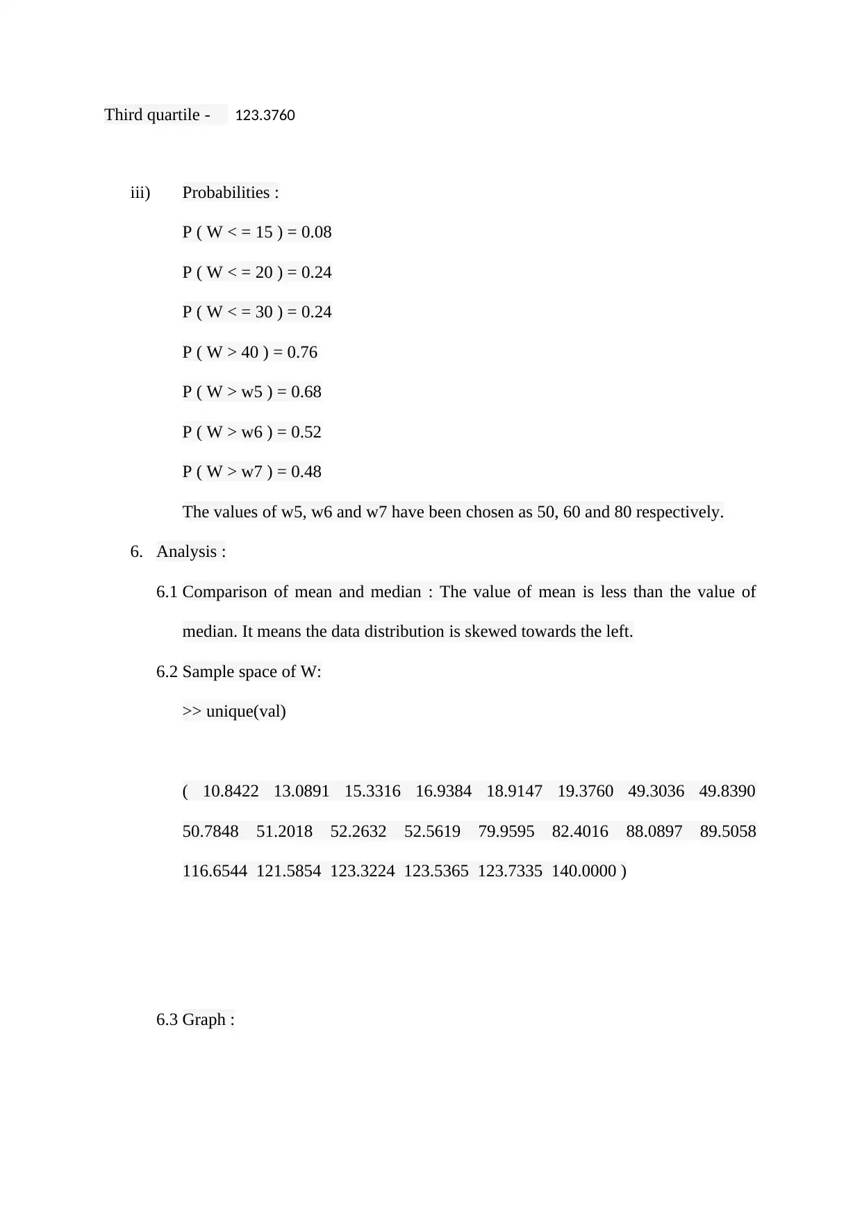
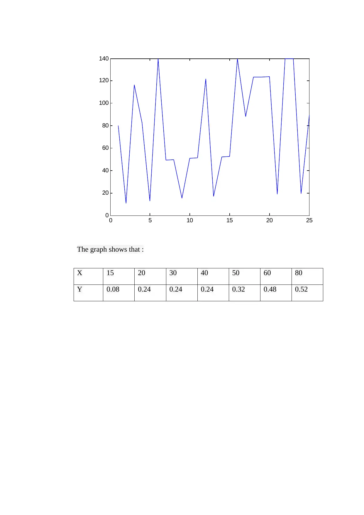
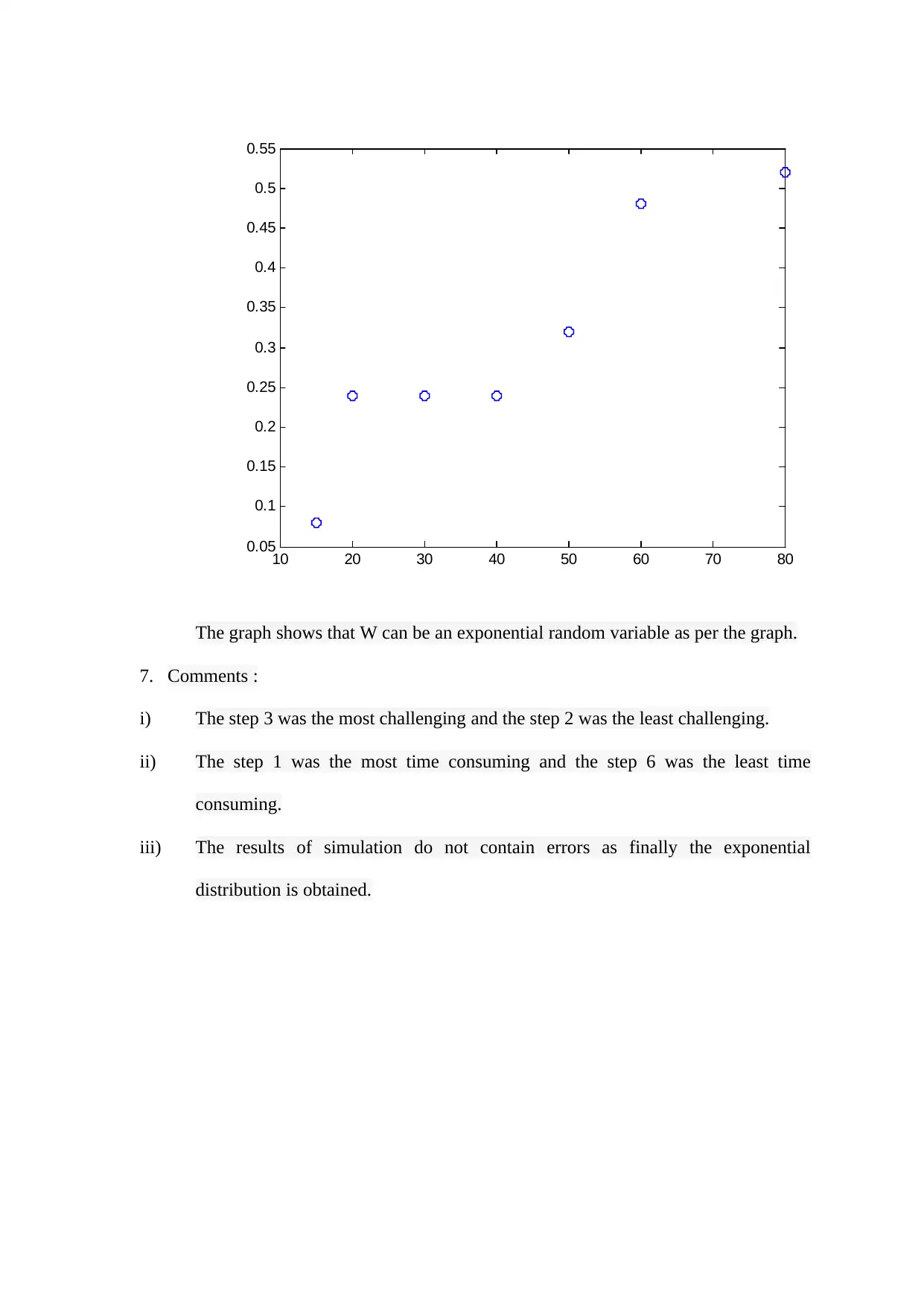
This project utilizes Monte-Carlo simulation to model a calling process. The student begins by generating random numbers using MATLAB and then formulates a model with defined notations for different actions like dialing, busy signals, and customer availability. The solution includes a detailed explanation of the cumulative distribution function for call duration, derivation of the inverse function, and a tree diagram representing the calling process. Data is collected through an ad-hoc experiment, and average values are calculated. The core of the project involves a Monte-Carlo simulation algorithm, considering two cases: customer answers and customer does not answer. The simulation runs for 1000 iterations, with results including mean, quartiles, and probabilities calculated for different time intervals. Analysis of the results compares the mean and median, discusses the distribution's skewness, and presents a graph indicating the potential exponential nature of the data. Finally, the student provides comments on the most and least challenging aspects of the project, along with a reflection on the accuracy of the simulation results.

Statistics
Student Name –
Student ID –
Random Number Generator ( using MATLAB ) :
The numbers u51 , u52 and u53 are 0.0628, 0.7091 and 0.0728 respectively as obtained by
the MATLAB code.
Simulation Problem :
1. Formulation of the model
1.1 Definition of notation :
The various elements of the model have been denoted as follows :
A : Turn on the phone and dial a number ( 6 seconds )
B: Detect a busy signal ( 3 seconds )
C: wait for 5 rings to conclude than no one will answer ( 25 seconds )
D: End the call ( 1 second )
E: Dialed 4 times
F: Customer is using the line ( P = 0.2 )
G: Customer is unavailable ( P = 0.3 )
H: Customer is available and can answer the call within X seconds
1.2 Cumulative distribution function of X :
X is a continuous random variable with the mean value of 12 seconds and the
exponential distribution.
Mean = m = 12

Parameter l = 1/m = 1/12
Cumulative distribution function = 1- e –lx , x >=0
And 0 , else
Hence, CDF = 1- e –x/12 , x >=0
And 0 , else
Expression for inverse :
F (x) = 1- e –x/12 ,
Hence, x = F-1 (u), u = (0,1)
F (x) – 1 = - e –x/12 ,
- F (x) + 1 = e –x/12 ,
-x/12 = ln (- F (x) + 1 )
X = -12 ln (1 – F(u))
Hence , the expression for inverse has been derived.
1.3 Tree diagram for the calling process :
A
Busy Ring
B C
4 times Pick
D
4 times done
F G H
END

2. Data Collection :
An ad – hoc experiment is performed using the phone. The time measurements are as
follows for the various tasks.
TASK -> A B C D H
1 7 2 24 1 8
2 5 3 22 1 10
3 5 3 25 1 12
4 4 2 21 1 14
5 5 1 22 1 6
6 4 2 24 1 8
7 4 1 24 1 10
8 5 2 24 1 9
9 5 2 22 1 11
10 6 2 22 1 12
Average 5 2 23 1 10
The average values found for the elements A, B , C, D and H are 5, 2, 23, 1 and 10 seconds
respectively.
3. Monte – Carlo Simulation Algorithm :
In the given simulation problem, W represents the total time which the representative
spends on calling 1 customer.
There are 2 cases here:
Case 1 : Customer answers the call –
The value of W can be found as follows :

0 unsuccessful calls : W = ( A + B + H ) = ( 6 + 3 + 12(1- e –x/12 )) = (9+12(1- e –x/12 ) )
1 unsuccessful calls : W = ( A + B + C + D ) + ( A + B + H ) = ( 6 + 3 + 25 + 1 ) + ( 6
+ 3 + 12(1- e –x/12 )) = 35 + (9+12(1- e –x/12 ) )
2 unsuccessful calls : W = 2 * ( A + B + C + D ) + ( A + B + H ) = 2 * ( 6 + 3 + 25 +
1 ) + ( 6 + 3 + 12(1- e –x/12 )) = 70 + (9+12(1- e –x/12 ) )
3 unsuccessful calls : W = 3 * ( A + B + C + D ) + ( A + B + H ) = 3 * ( 6 + 3 + 25 +
1 ) + ( 6 + 3 + 12(1- e –x/12 )) = 105 + (9+12(1- e –x/12 ) )
Case 2 : Customer does not answer the call –
The value of W can be found as follows :
W = 4 * ( A + B + C + D ) = 4 * ( 6 + 3 + 25 + 1 ) = 4*35 = 140
4. Simulation :
The process is simulated 1000 times
5. Estimation :
i) Mean -
76.3694
ii) First quartile - 41.8217
Median - 79.9595

Third quartile - 123.3760
iii) Probabilities :
P ( W < = 15 ) = 0.08
P ( W < = 20 ) = 0.24
P ( W < = 30 ) = 0.24
P ( W > 40 ) = 0.76
P ( W > w5 ) = 0.68
P ( W > w6 ) = 0.52
P ( W > w7 ) = 0.48
The values of w5, w6 and w7 have been chosen as 50, 60 and 80 respectively.
6. Analysis :
6.1 Comparison of mean and median : The value of mean is less than the value of
median. It means the data distribution is skewed towards the left.
6.2 Sample space of W:
>> unique(val)
( 10.8422 13.0891 15.3316 16.9384 18.9147 19.3760 49.3036 49.8390
50.7848 51.2018 52.2632 52.5619 79.9595 82.4016 88.0897 89.5058
116.6544 121.5854 123.3224 123.5365 123.7335 140.0000 )
6.3 Graph :

0 5 10 15 20 25
0
20
40
60
80
100
120
140
The graph shows that :
X 15 20 30 40 50 60 80
Y 0.08 0.24 0.24 0.24 0.32 0.48 0.52

10 20 30 40 50 60 70 80
0.05
0.1
0.15
0.2
0.25
0.3
0.35
0.4
0.45
0.5
0.55
The graph shows that W can be an exponential random variable as per the graph.
7. Comments :
i) The step 3 was the most challenging and the step 2 was the least challenging.
ii) The step 1 was the most time consuming and the step 6 was the least time
consuming.
iii) The results of simulation do not contain errors as finally the exponential
distribution is obtained.