Handbook of Differential Equation
VerifiedAdded on 2022/09/08
|12
|940
|27
AI Summary
Contribute Materials
Your contribution can guide someone’s learning journey. Share your
documents today.
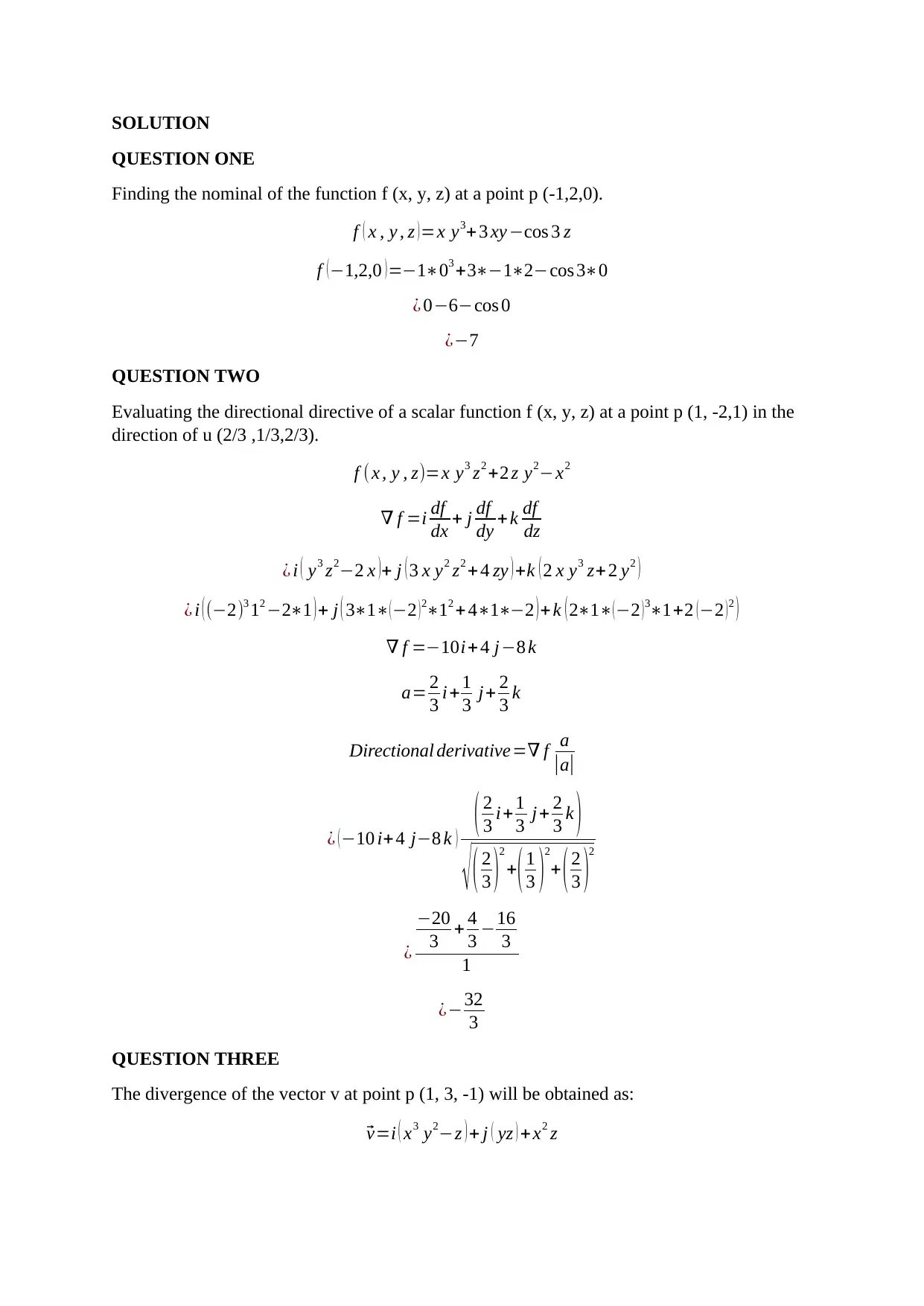
SOLUTION
QUESTION ONE
Finding the nominal of the function f (x, y, z) at a point p (-1,2,0).
f ( x , y , z )=x y3+ 3 xy −cos 3 z
f (−1,2,0 )=−1∗03 +3∗−1∗2−cos 3∗0
¿ 0−6−cos 0
¿−7
QUESTION TWO
Evaluating the directional directive of a scalar function f (x, y, z) at a point p (1, -2,1) in the
direction of u (2/3 ,1/3,2/3).
f ( x , y , z)=x y3 z2 +2 z y2−x2
∇ f =i df
dx + j df
dy + k df
dz
¿ i ( y3 z2−2 x )+ j ( 3 x y2 z2 +4 zy ) +k ( 2 x y3 z+ 2 y2 )
¿ i ( (−2)3 12 −2∗1 ) + j ( 3∗1∗( −2 ) 2∗12 + 4∗1∗−2 ) +k ( 2∗1∗( −2 ) 3∗1+2 ( −2 ) 2 )
∇ f =−10i+ 4 j−8 k
a= 2
3 i+ 1
3 j+ 2
3 k
Directional derivative=∇ f a
|a|
¿ (−10 i+4 j−8 k ) ( 2
3 i+ 1
3 j+ 2
3 k )
√ ( 2
3 )2
+( 1
3 )2
+ ( 2
3 )2
¿
−20
3 + 4
3 −16
3
1
¿−32
3
QUESTION THREE
The divergence of the vector v at point p (1, 3, -1) will be obtained as:⃗
v=i ( x3 y2−z ) + j ( yz ) +x2 z
Secure Best Marks with AI Grader
Need help grading? Try our AI Grader for instant feedback on your assignments.
¿ (⃗ v )= d⃗ v1
dx + d⃗ v2
dy + d⃗ v3
dz
¿ 3 x2+ z +x2
¿ 3 ¿ 12−1+ (−1 )2=3
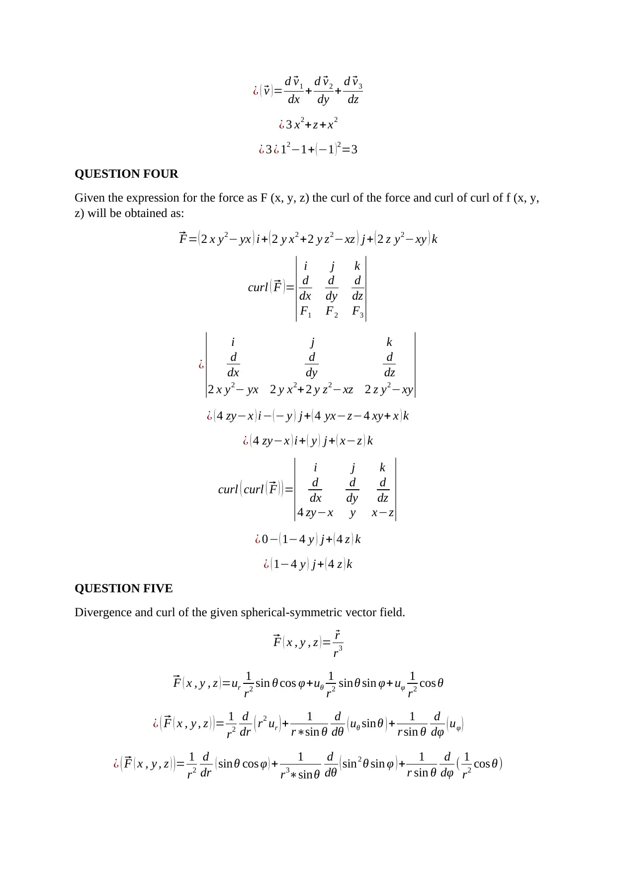
QUESTION FOUR
Given the expression for the force as F (x, y, z) the curl of the force and curl of curl of f (x, y,
z) will be obtained as:⃗
F= ( 2 x y2− yx ) i+ ( 2 y x2 +2 y z2−xz ) j+ ( 2 z y2−xy ) k
curl (⃗ F )=
| i j k
d
dx
d
dy
d
dz
F1 F2 F3
|
¿
| i j k
d
dx
d
dy
d
dz
2 x y2− yx 2 y x2+2 y z2−xz 2 z y2−xy
|
¿ ( 4 zy−x ) i− (− y ) j+ ( 4 yx−z−4 xy+ x ) k
¿ ( 4 zy−x ) i+ ( y ) j+ ( x−z ) k
curl ( curl (⃗ F ) )=
| i j k
d
dx
d
dy
d
dz
4 zy−x y x−z
|
¿ 0− ( 1−4 y ) j+ ( 4 z ) k
¿ ( 1−4 y ) j+ ( 4 z ) k
QUESTION FIVE
Divergence and curl of the given spherical-symmetric vector field.⃗
F ( x , y , z )=⃗ r
r3⃗
F ( x , y , z )=ur
1
r2 sin θ cos φ+uθ
1
r2 sinθ sin φ+ uφ
1
r2 cos θ
¿ (⃗ F ( x , y , z ) )= 1
r2
d
dr ( r2 ur )+ 1
r∗sin θ
d
dθ ( uθ sinθ ) + 1
r sin θ
d
dφ ( uφ )
¿ (⃗ F ( x , y , z ) )= 1
r2
d
dr ( sinθ cos φ ) + 1
r3∗sinθ
d
dθ ( sin2 θ sin φ ) + 1
r sin θ
d
dφ ( 1
r2 cos θ)
dx + d⃗ v2
dy + d⃗ v3
dz
¿ 3 x2+ z +x2
¿ 3 ¿ 12−1+ (−1 )2=3
QUESTION FOUR
Given the expression for the force as F (x, y, z) the curl of the force and curl of curl of f (x, y,
z) will be obtained as:⃗
F= ( 2 x y2− yx ) i+ ( 2 y x2 +2 y z2−xz ) j+ ( 2 z y2−xy ) k
curl (⃗ F )=
| i j k
d
dx
d
dy
d
dz
F1 F2 F3
|
¿
| i j k
d
dx
d
dy
d
dz
2 x y2− yx 2 y x2+2 y z2−xz 2 z y2−xy
|
¿ ( 4 zy−x ) i− (− y ) j+ ( 4 yx−z−4 xy+ x ) k
¿ ( 4 zy−x ) i+ ( y ) j+ ( x−z ) k
curl ( curl (⃗ F ) )=
| i j k
d
dx
d
dy
d
dz
4 zy−x y x−z
|
¿ 0− ( 1−4 y ) j+ ( 4 z ) k
¿ ( 1−4 y ) j+ ( 4 z ) k
QUESTION FIVE
Divergence and curl of the given spherical-symmetric vector field.⃗
F ( x , y , z )=⃗ r
r3⃗
F ( x , y , z )=ur
1
r2 sin θ cos φ+uθ
1
r2 sinθ sin φ+ uφ
1
r2 cos θ
¿ (⃗ F ( x , y , z ) )= 1
r2
d
dr ( r2 ur )+ 1
r∗sin θ
d
dθ ( uθ sinθ ) + 1
r sin θ
d
dφ ( uφ )
¿ (⃗ F ( x , y , z ) )= 1
r2
d
dr ( sinθ cos φ ) + 1
r3∗sinθ
d
dθ ( sin2 θ sin φ ) + 1
r sin θ
d
dφ ( 1
r2 cos θ)
¿ (⃗ F ( x , y , z ) )=0+ 1
r3∗sin θ 2cos θ sin θ+ 0
¿ (⃗ F ( x , y , z ) )= 1
r3 2cos θ
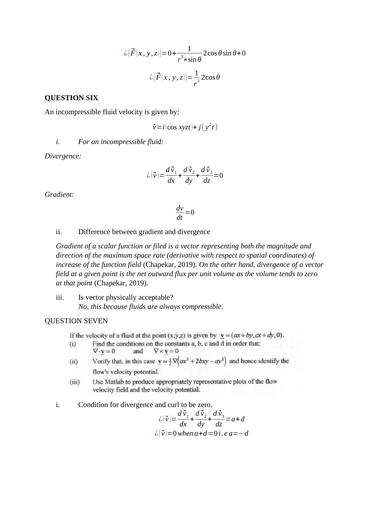
QUESTION SIX
An incompressible fluid velocity is given by:⃗
v=i ( cos xyzt )+ j( y2 t )
i. For an incompressible fluid:
Divergence:
¿ (⃗ v ) = d⃗ v1
dx + d⃗ v2
dy + d⃗ v3
dz =0
Gradient:
dv
dt =0
ii. Difference between gradient and divergence
Gradient of a scalar function or filed is a vector representing both the magnitude and
direction of the maximum space rate (derivative with respect to spatial coordinates) of
increase of the function field (Chapekar, 2019). On the other hand, divergence of a vector
field at a given point is the net outward flux per unit volume as the volume tends to zero
at that point (Chapekar, 2019).
iii. Is vector physically acceptable?
No, this because fluids are always compressible.
QUESTION SEVEN
i. Condition for divergence and curl to be zero.
¿ (⃗ v ) = d⃗ v1
dx + d⃗ v2
dy + d⃗ v3
dz =a+d
¿ (⃗ v ) =0 when a+d =0 i. e a=−d
r3∗sin θ 2cos θ sin θ+ 0
¿ (⃗ F ( x , y , z ) )= 1
r3 2cos θ
QUESTION SIX
An incompressible fluid velocity is given by:⃗
v=i ( cos xyzt )+ j( y2 t )
i. For an incompressible fluid:
Divergence:
¿ (⃗ v ) = d⃗ v1
dx + d⃗ v2
dy + d⃗ v3
dz =0
Gradient:
dv
dt =0
ii. Difference between gradient and divergence
Gradient of a scalar function or filed is a vector representing both the magnitude and
direction of the maximum space rate (derivative with respect to spatial coordinates) of
increase of the function field (Chapekar, 2019). On the other hand, divergence of a vector
field at a given point is the net outward flux per unit volume as the volume tends to zero
at that point (Chapekar, 2019).
iii. Is vector physically acceptable?
No, this because fluids are always compressible.
QUESTION SEVEN
i. Condition for divergence and curl to be zero.
¿ (⃗ v ) = d⃗ v1
dx + d⃗ v2
dy + d⃗ v3
dz =a+d
¿ (⃗ v ) =0 when a+d =0 i. e a=−d
curl ( curl (⃗ F ) ) =
| i j k
d
dx
d
dy
d
dz
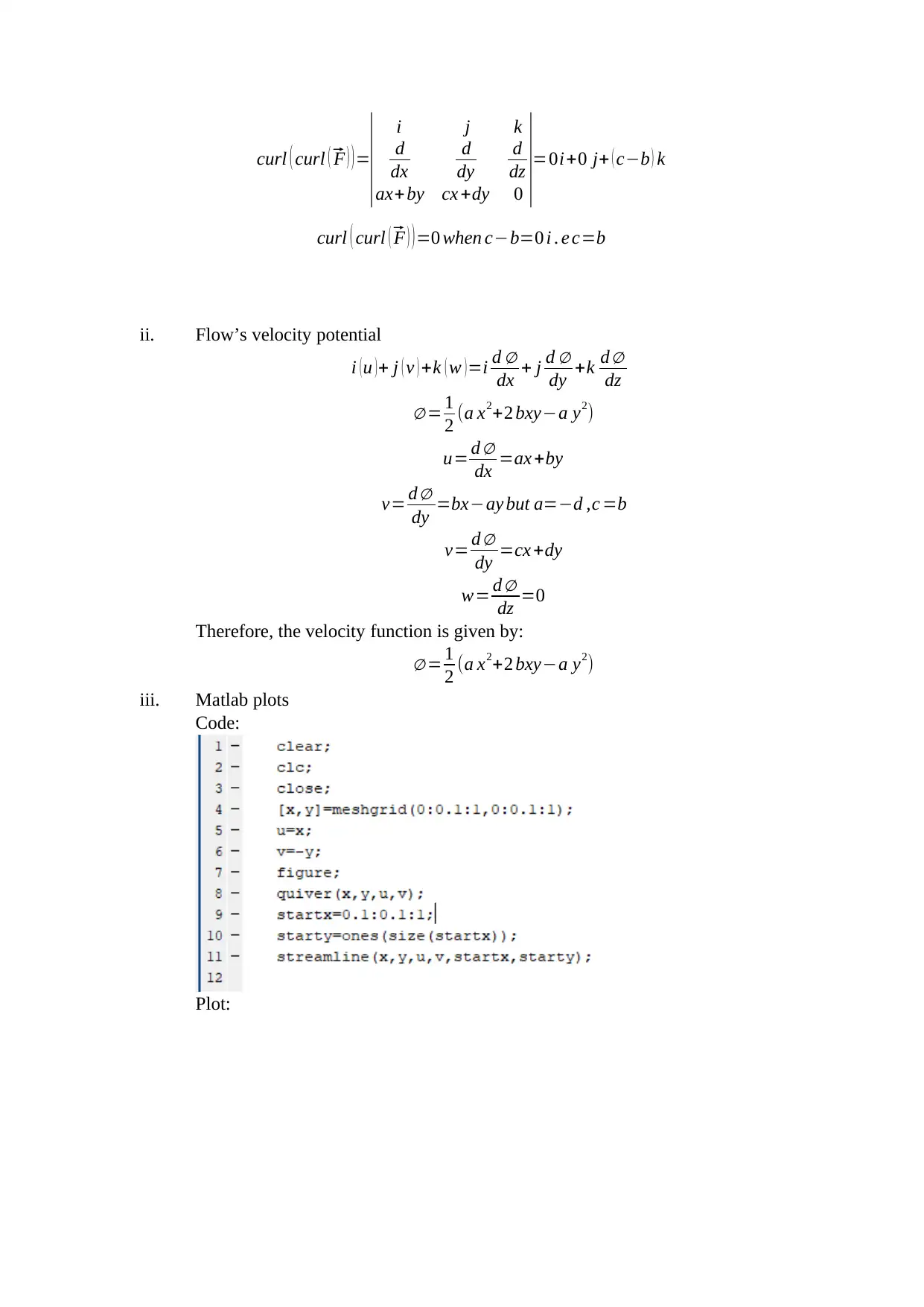
ax+ by cx +dy 0 |=0i+0 j+ ( c−b ) k
curl ( curl (⃗ F ) )=0 when c−b=0 i . e c=b
ii. Flow’s velocity potential
i (u )+ j ( v ) +k ( w )=i d ∅
dx + j d ∅
dy +k d ∅
dz
∅ = 1
2 (a x2+2 bxy−a y2)
u= d ∅
dx =ax +by
v= d ∅
dy =bx−ay but a=−d ,c =b
v= d ∅
dy =cx +dy
w= d ∅
dz =0
Therefore, the velocity function is given by:
∅ = 1
2 (a x2+2 bxy−a y2)
iii. Matlab plots
Code:
Plot:
| i j k
d
dx
d
dy
d
dz
ax+ by cx +dy 0 |=0i+0 j+ ( c−b ) k
curl ( curl (⃗ F ) )=0 when c−b=0 i . e c=b
ii. Flow’s velocity potential
i (u )+ j ( v ) +k ( w )=i d ∅
dx + j d ∅
dy +k d ∅
dz
∅ = 1
2 (a x2+2 bxy−a y2)
u= d ∅
dx =ax +by
v= d ∅
dy =bx−ay but a=−d ,c =b
v= d ∅
dy =cx +dy
w= d ∅
dz =0
Therefore, the velocity function is given by:
∅ = 1
2 (a x2+2 bxy−a y2)
iii. Matlab plots
Code:
Plot:
Secure Best Marks with AI Grader
Need help grading? Try our AI Grader for instant feedback on your assignments.
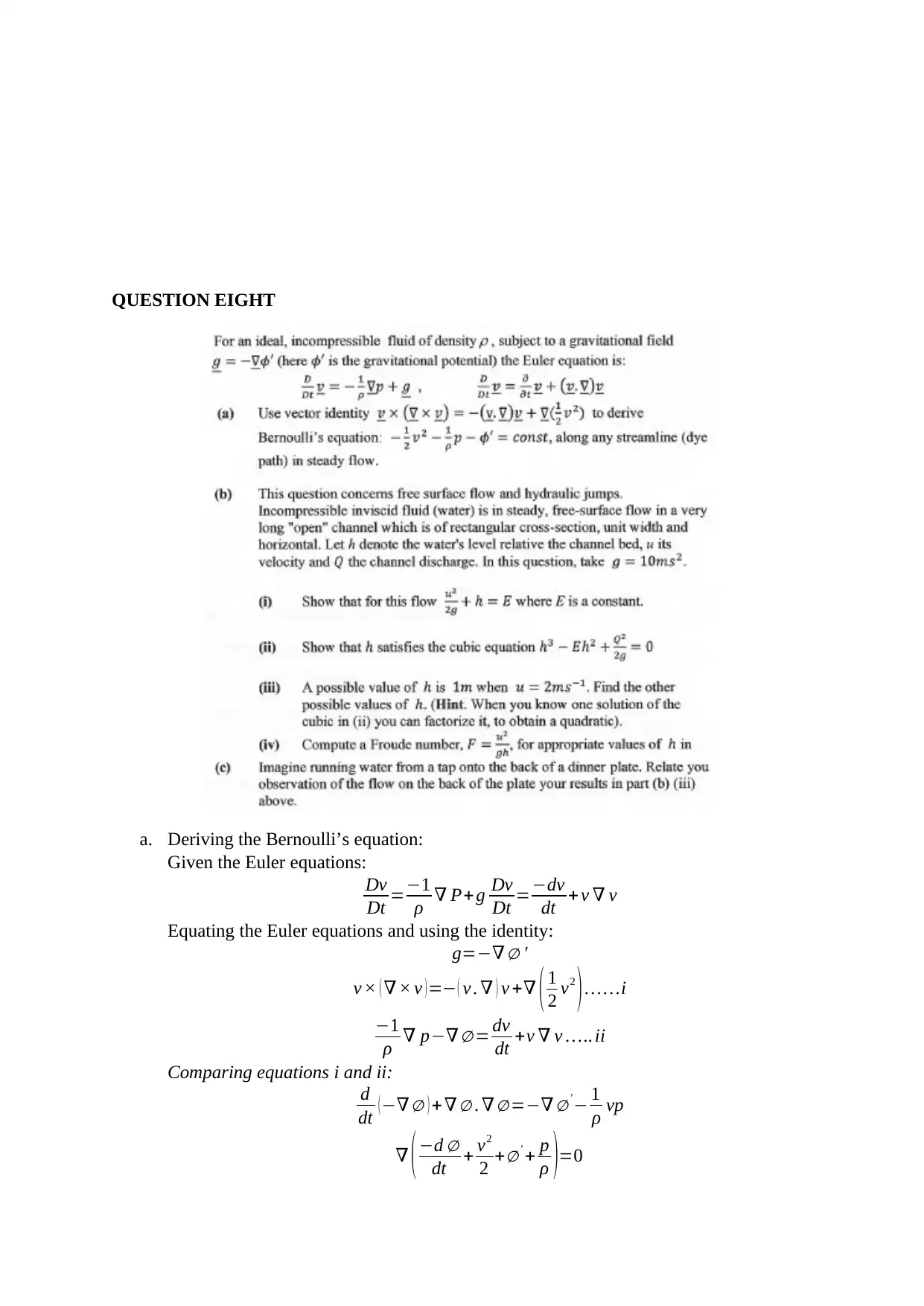
QUESTION EIGHT
a. Deriving the Bernoulli’s equation:
Given the Euler equations:
Dv
Dt =−1
ρ ∇ P+ g Dv
Dt =−dv
dt +v ∇ v
Equating the Euler equations and using the identity:
g=−∇ ∅ '
v × ( ∇ × v )=− ( v . ∇ ) v +∇ ( 1
2 v2
)… …i
−1
ρ ∇ p−∇ ∅ = dv
dt +v ∇ v ….. ii
Comparing equations i and ii:
d
dt ( −∇ ∅ ) +∇ ∅ . ∇ ∅ =−∇ ∅ '− 1
ρ vp
∇ (−d ∅
dt + v2
2 +∅' + p
ρ )=0
−d ∅
dt + v2
2 +∅ ' + p
ρ =constant
v2
2 +∅ ' + p
ρ =constant
Therefore :
−1
2 v2 − 1
ρ p−∅' =constant
b. Surface flow and hydraulic jumps
i. Proving the flow.
po
p + 1
2 u2 +gh=constant
Given the system po
p is constant.
1
2 u2 + gh=constant
Dividing everywhere by g:
u2
2 g +h−E=0
ii. Cubic equation
u2
2 g +h−E=0 … …i
Q=v∗h→ Q2=v2∗h2
Multiplying everywhere by h2:
u2 h2
2 g +h3 −E h2=0
Q2
2 g +h3 −E h2=0
iii. Finding the values of h:
u2 h2
2 g +h3 −E h2
h2
( u2
2 g + h−E )=0
h2 =0∧h=−u2
2 g + E=1
h=0
iv. Finding the other value of h that satisfies the equation
F= u2
gh = 22
10∗1 =0.4
c. Relating the results in b.
The flow will not be in streamline and therefore:
Q2
2 g +h3 −E h2=0
QUESTION NINE
Solution to the system of coupled differential equation:
[ dx
dt
dy
dt ] =
[ −6 2
−1 −3 ][ x
y ]
The general solution for the coupled differential equation is given by:
( x , y ) =( A , B) e λt
[ [ −6 2
−1 −3 ] −λ [ 1 0
0 1 ] ] [ A
B ]=0
[ −6−λ 2
−1 −3−λ ][ A
B ] =0
But the matrix with A and B cannot be equal to zero. Therefore:
[ −6−λ 2
−1 −3−λ ]=0
(−6−λ ) (−3−λ )+2=0
λ=−4 , λ=−5
When λ=−4
[−2 2
−1 1 ][ A
B ]=0∧therefore [ A
B ]=α [ 1
−1 ]
When λ=−5
[−1 2
−1 2 ][ A
B ]=0∧therefore [ A
B ]=β [ 1
1
2 ]
The general solution is:
[ x (t )
y (t) ]=α [ 1
−1 ]e−4 t +β [ 1
1
2 ]e−5 t
Substituting for the initial conditions to the values of alpha and beta.
[ x ( 0 )
y ( 0 ) ]= [ 1
−2 ]=α [ 1
−1 ]+ β [ 1
1
2 ]
[ 1 1
−2 −1 ][ α
β ] =
[ 1
−2 ]
Paraphrase This Document
Need a fresh take? Get an instant paraphrase of this document with our AI Paraphraser
[ α
β ]=
[ 5
3
−2
3 ]
[ x (t )
y (t) ]=5
3 [ 1
−1 ]e−4 t − 2
3 [ 1
1
2 ]e−5 t
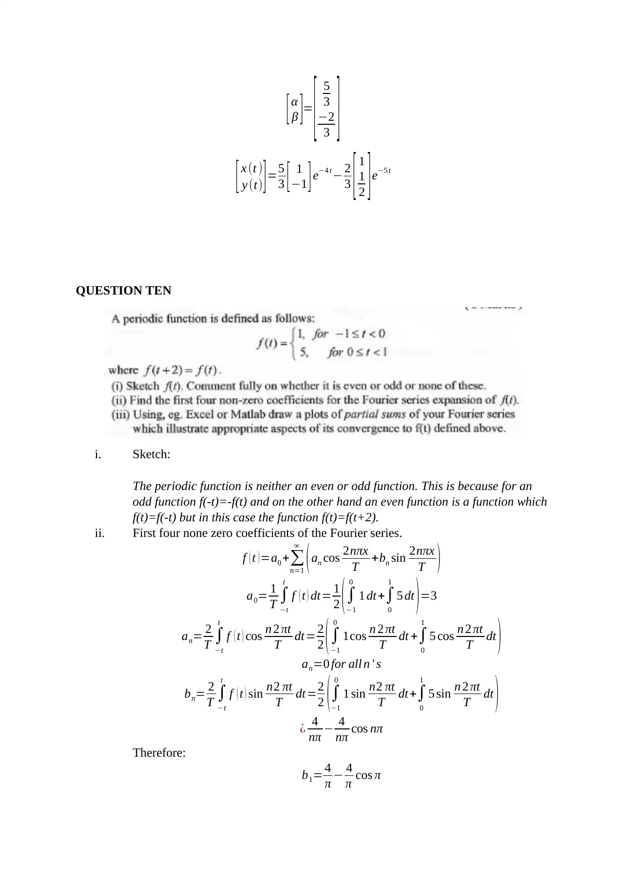
QUESTION TEN
i. Sketch:
The periodic function is neither an even or odd function. This is because for an
odd function f(-t)=-f(t) and on the other hand an even function is a function which
f(t)=f(-t) but in this case the function f(t)=f(t+2).
ii. First four none zero coefficients of the Fourier series.
f ( t )=a0 +∑
n=1
∞
(an cos 2nπx
T +bn sin 2nπx
T )
a0= 1
T ∫
−t
t
f ( t ) dt= 1
2 (∫
−1
0
1 dt+∫
0
1
5 dt )=3
an= 2
T ∫
−t
t
f ( t ) cos n 2 πt
T dt= 2
2 (∫
−1
0
1cos n 2 πt
T dt +∫
0
1
5 cos n 2 πt
T dt )
an=0 for all n ' s
bn= 2
T ∫
−t
t
f ( t ) sin n2 πt
T dt=2
2 (∫
−1
0
1 sin n2 πt
T dt+∫
0
1
5 sin n 2 πt
T dt )
¿ 4
nπ − 4
nπ cos nπ
Therefore:
b1= 4
π − 4
π cos π
β ]=
[ 5
3
−2
3 ]
[ x (t )
y (t) ]=5
3 [ 1
−1 ]e−4 t − 2
3 [ 1
1
2 ]e−5 t
QUESTION TEN
i. Sketch:
The periodic function is neither an even or odd function. This is because for an
odd function f(-t)=-f(t) and on the other hand an even function is a function which
f(t)=f(-t) but in this case the function f(t)=f(t+2).
ii. First four none zero coefficients of the Fourier series.
f ( t )=a0 +∑
n=1
∞
(an cos 2nπx
T +bn sin 2nπx
T )
a0= 1
T ∫
−t
t
f ( t ) dt= 1
2 (∫
−1
0
1 dt+∫
0
1
5 dt )=3
an= 2
T ∫
−t
t
f ( t ) cos n 2 πt
T dt= 2
2 (∫
−1
0
1cos n 2 πt
T dt +∫
0
1
5 cos n 2 πt
T dt )
an=0 for all n ' s
bn= 2
T ∫
−t
t
f ( t ) sin n2 πt
T dt=2
2 (∫
−1
0
1 sin n2 πt
T dt+∫
0
1
5 sin n 2 πt
T dt )
¿ 4
nπ − 4
nπ cos nπ
Therefore:
b1= 4
π − 4
π cos π
b2= 4
2 π − 4
2 π cos 2 π
b3= 4
3 π − 4
3 π cos 3 π
b4= 4
4 π − 4
4 π cos 4 π
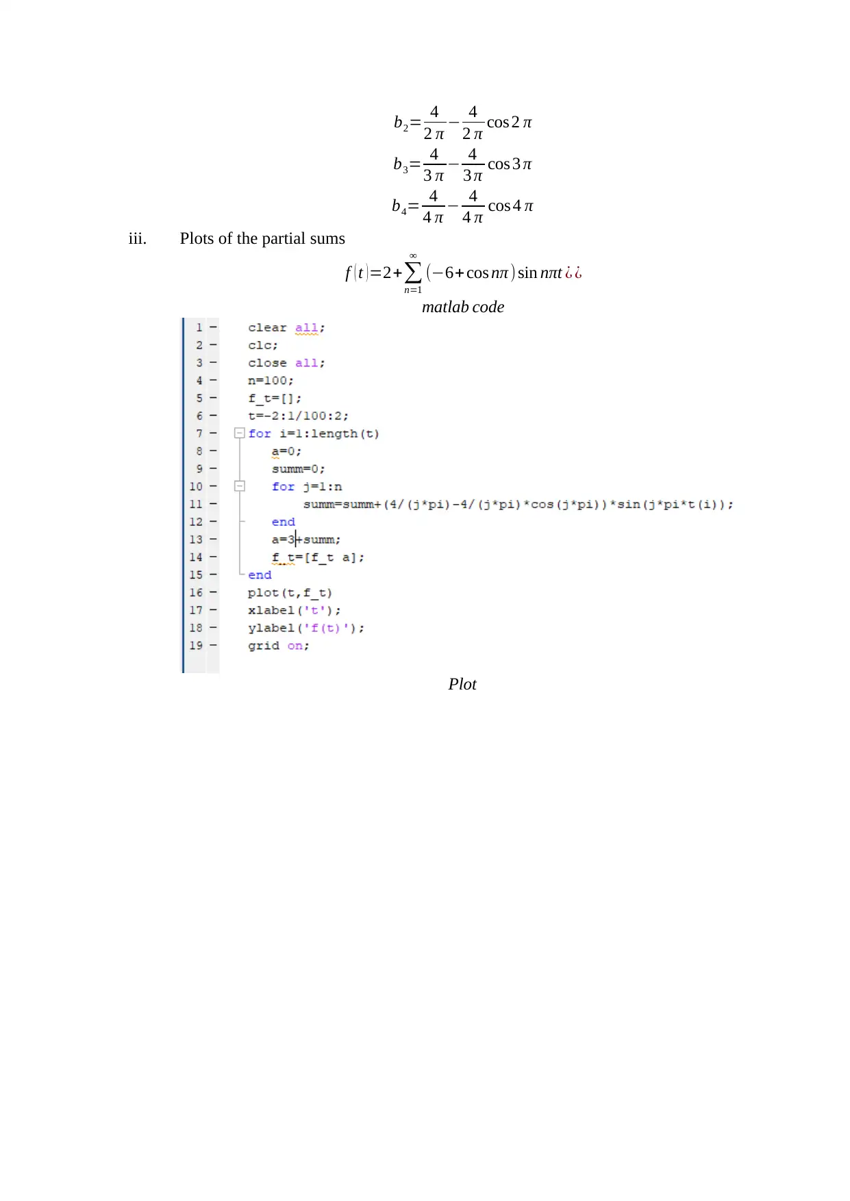
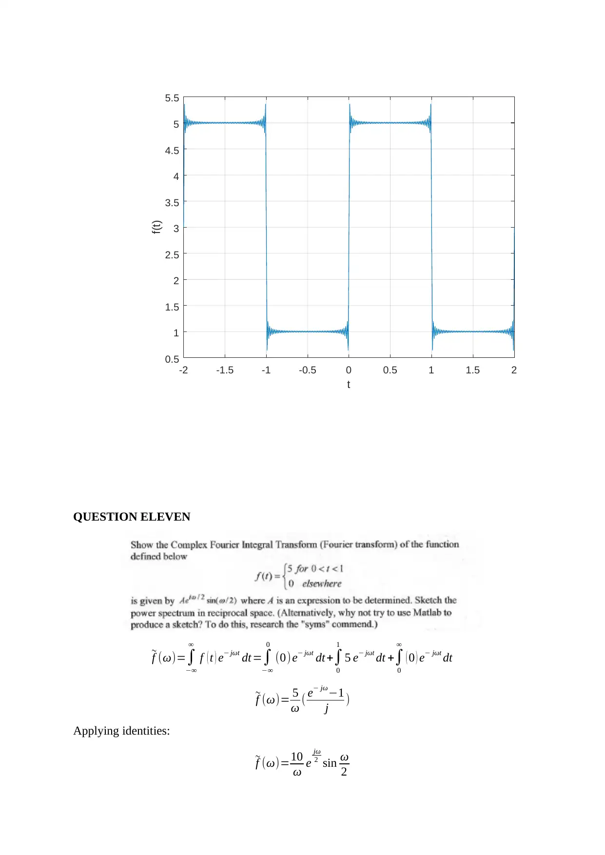
iii. Plots of the partial sums
f ( t )=2+∑
n=1
∞
(−6+ cos nπ ) sin nπt ¿ ¿
matlab code
Plot
2 π − 4
2 π cos 2 π
b3= 4
3 π − 4
3 π cos 3 π
b4= 4
4 π − 4
4 π cos 4 π
iii. Plots of the partial sums
f ( t )=2+∑
n=1
∞
(−6+ cos nπ ) sin nπt ¿ ¿
matlab code
Plot
-2 -1.5 -1 -0.5 0 0.5 1 1.5 2
t
0.5
1
1.5
2
2.5
3
3.5
4
4.5
5
5.5
f(t)
QUESTION ELEVEN
~
f (ω)=∫
−∞
∞
f ( t ) e− jωt dt=∫
−∞
0
(0) e− jωt dt+∫
0
1
5 e− jωt dt +∫
0
∞
( 0 ) e− jωt dt
~
f (ω)= 5
ω ( e− jω−1
j )
Applying identities:
~
f (ω)=10
ω e
jω
2 sin ω
2
t
0.5
1
1.5
2
2.5
3
3.5
4
4.5
5
5.5
f(t)
QUESTION ELEVEN
~
f (ω)=∫
−∞
∞
f ( t ) e− jωt dt=∫
−∞
0
(0) e− jωt dt+∫
0
1
5 e− jωt dt +∫
0
∞
( 0 ) e− jωt dt
~
f (ω)= 5
ω ( e− jω−1
j )
Applying identities:
~
f (ω)=10
ω e
jω
2 sin ω
2
Secure Best Marks with AI Grader
Need help grading? Try our AI Grader for instant feedback on your assignments.
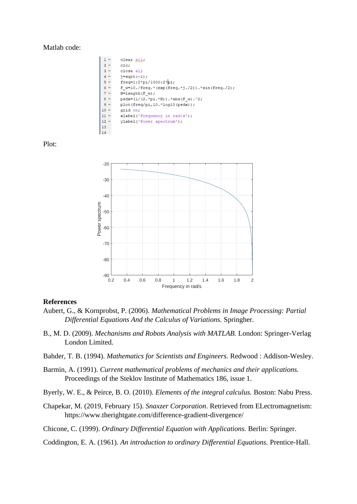
Matlab code:
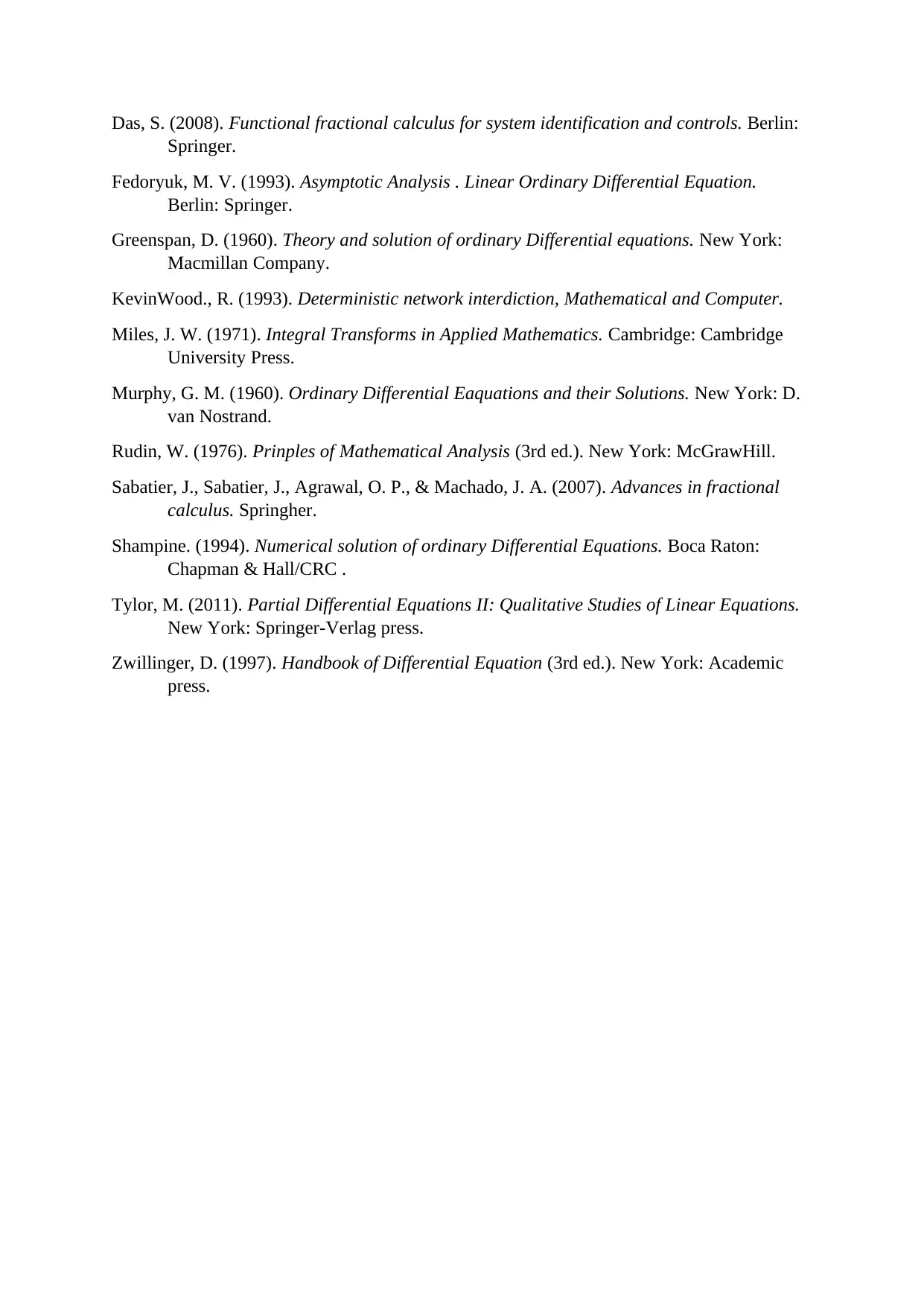
Plot:
0.2 0.4 0.6 0.8 1 1.2 1.4 1.6 1.8 2
Frequency in rad/s
-90
-80
-70
-60
-50
-40
-30
-20
Power spectrum
References
Aubert, G., & Kornprobst, P. (2006). Mathematical Problems in Image Processing: Partial
Differential Equations And the Calculus of Variations. Springher.
B., M. D. (2009). Mechanisms and Robots Analysis with MATLAB. London: Springer-Verlag
London Limited.
Bahder, T. B. (1994). Mathematics for Scientists and Engineers. Redwood : Addison-Wesley.
Barmin, A. (1991). Current mathematical problems of mechanics and their applications.
Proceedings of the Steklov Institute of Mathematics 186, issue 1.
Byerly, W. E., & Peirce, B. O. (2010). Elements of the integral calculus. Boston: Nabu Press.
Chapekar, M. (2019, February 15). Snaxzer Corporation. Retrieved from ELectromagnetism:
https://www.therightgate.com/difference-gradient-divergence/
Chicone, C. (1999). Ordinary Differential Equation with Applications. Berlin: Springer.
Coddington, E. A. (1961). An introduction to ordinary Differential Equations. Prentice-Hall.
Das, S. (2008). Functional fractional calculus for system identification and controls. Berlin:
Springer.
Fedoryuk, M. V. (1993). Asymptotic Analysis . Linear Ordinary Differential Equation.
Berlin: Springer.
Greenspan, D. (1960). Theory and solution of ordinary Differential equations. New York:
Macmillan Company.
KevinWood., R. (1993). Deterministic network interdiction, Mathematical and Computer.
Miles, J. W. (1971). Integral Transforms in Applied Mathematics. Cambridge: Cambridge
University Press.
Murphy, G. M. (1960). Ordinary Differential Eaquations and their Solutions. New York: D.
van Nostrand.
Rudin, W. (1976). Prinples of Mathematical Analysis (3rd ed.). New York: McGrawHill.
Sabatier, J., Sabatier, J., Agrawal, O. P., & Machado, J. A. (2007). Advances in fractional
calculus. Springher.
Shampine. (1994). Numerical solution of ordinary Differential Equations. Boca Raton:
Chapman & Hall/CRC .
Tylor, M. (2011). Partial Differential Equations II: Qualitative Studies of Linear Equations.
New York: Springer-Verlag press.
Zwillinger, D. (1997). Handbook of Differential Equation (3rd ed.). New York: Academic
press.
1 out of 12
Related Documents


Your All-in-One AI-Powered Toolkit for Academic Success.
+13062052269
info@desklib.com
Available 24*7 on WhatsApp / Email
![[object Object]](/_next/static/media/star-bottom.7253800d.svg)
Unlock your academic potential
© 2024 | Zucol Services PVT LTD | All rights reserved.