STATS 201/8 Assignment 2: Cholesterol, Diamonds, and FDG
VerifiedAdded on 2022/09/14
|12
|2427
|14
Homework Assignment
AI Summary
This assignment solution for STATS 201/8 involves analyzing three different datasets using R programming. The first part focuses on comparing cholesterol intake between male and female students, examining both mean and median values using t-tests and boxplots. The second part investigates the relationship between diamond color and price using linear regression. The final part analyzes FDG scores to determine if they differ between normal individuals and Alzheimer's disease patients, considering the effect of age, and utilizes prediction intervals. The solution includes data inspection, model fitting, assumption checks, and executive summaries for each question. The student has used statistical methods and R programming to answer the questions and provide interpretations of the findings.
STATS 201/8 Assignment 2
Your name and ID here
Due Date: 3pm Thursday 29th October
Question 1
Question of interest/goal of the study
We want to compare both the mean and median cholesterol intake for male and female students.
Read in and inspect the data:
chol.df=read.table("chol.txt",header=TRUE)
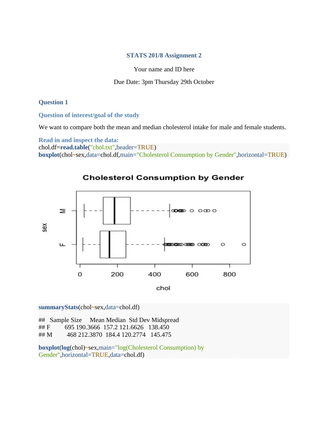
boxplot(chol~sex,data=chol.df,main="Cholesterol Consumption by Gender",horizontal=TRUE)
summaryStats(chol~sex,data=chol.df)
## Sample Size Mean Median Std Dev Midspread
## F 695 190.3666 157.2 121.6626 138.450
## M 468 212.3870 184.4 120.2774 145.475
boxplot(log(chol)~sex,main="log(Cholesterol Consumption) by
Gender",horizontal=TRUE,data=chol.df)
Your name and ID here
Due Date: 3pm Thursday 29th October
Question 1
Question of interest/goal of the study
We want to compare both the mean and median cholesterol intake for male and female students.
Read in and inspect the data:
chol.df=read.table("chol.txt",header=TRUE)
boxplot(chol~sex,data=chol.df,main="Cholesterol Consumption by Gender",horizontal=TRUE)
summaryStats(chol~sex,data=chol.df)
## Sample Size Mean Median Std Dev Midspread
## F 695 190.3666 157.2 121.6626 138.450
## M 468 212.3870 184.4 120.2774 145.475
boxplot(log(chol)~sex,main="log(Cholesterol Consumption) by
Gender",horizontal=TRUE,data=chol.df)
Paraphrase This Document
Need a fresh take? Get an instant paraphrase of this document with our AI Paraphraser
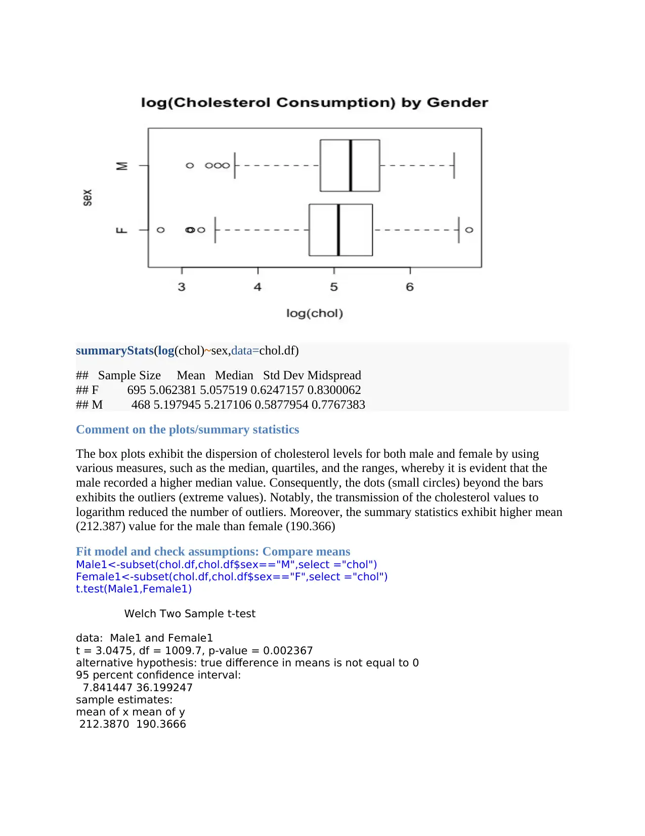
summaryStats(log(chol)~sex,data=chol.df)
## Sample Size Mean Median Std Dev Midspread
## F 695 5.062381 5.057519 0.6247157 0.8300062
## M 468 5.197945 5.217106 0.5877954 0.7767383
Comment on the plots/summary statistics
The box plots exhibit the dispersion of cholesterol levels for both male and female by using
various measures, such as the median, quartiles, and the ranges, whereby it is evident that the
male recorded a higher median value. Consequently, the dots (small circles) beyond the bars
exhibits the outliers (extreme values). Notably, the transmission of the cholesterol values to
logarithm reduced the number of outliers. Moreover, the summary statistics exhibit higher mean
(212.387) value for the male than female (190.366)
Fit model and check assumptions: Compare means
Male1<-subset(chol.df,chol.df$sex=="M",select ="chol")
Female1<-subset(chol.df,chol.df$sex=="F",select ="chol")
t.test(Male1,Female1)
Welch Two Sample t-test
data: Male1 and Female1
t = 3.0475, df = 1009.7, p-value = 0.002367
alternative hypothesis: true difference in means is not equal to 0
95 percent confidence interval:
7.841447 36.199247
sample estimates:
mean of x mean of y
212.3870 190.3666
As evident, the p-value (0.002367) is less than the significance level (0.05) thus there is
difference between the means for both gender (sex)
Fit model and check assumptions: Compare medians
Female<-c(rnorm(695,157.2,121.6626))
Male<-c(rnorm(468,184.4,120.2774))
t.test(Female, Male, paired = FALSE)
Welch Two Sample t-test
data: Female and Male
t = -4.4069, df = 1010.9, p-value =
1.161e-05
alternative hypothesis: true difference in means is not equal to 0
95 percent confidence interval:
-46.09315 -17.69110
As evident, the p-value (1.161e-05) is less than the significance level thus there is difference
between the means for both gender (sex).
Method and Assumption Checks
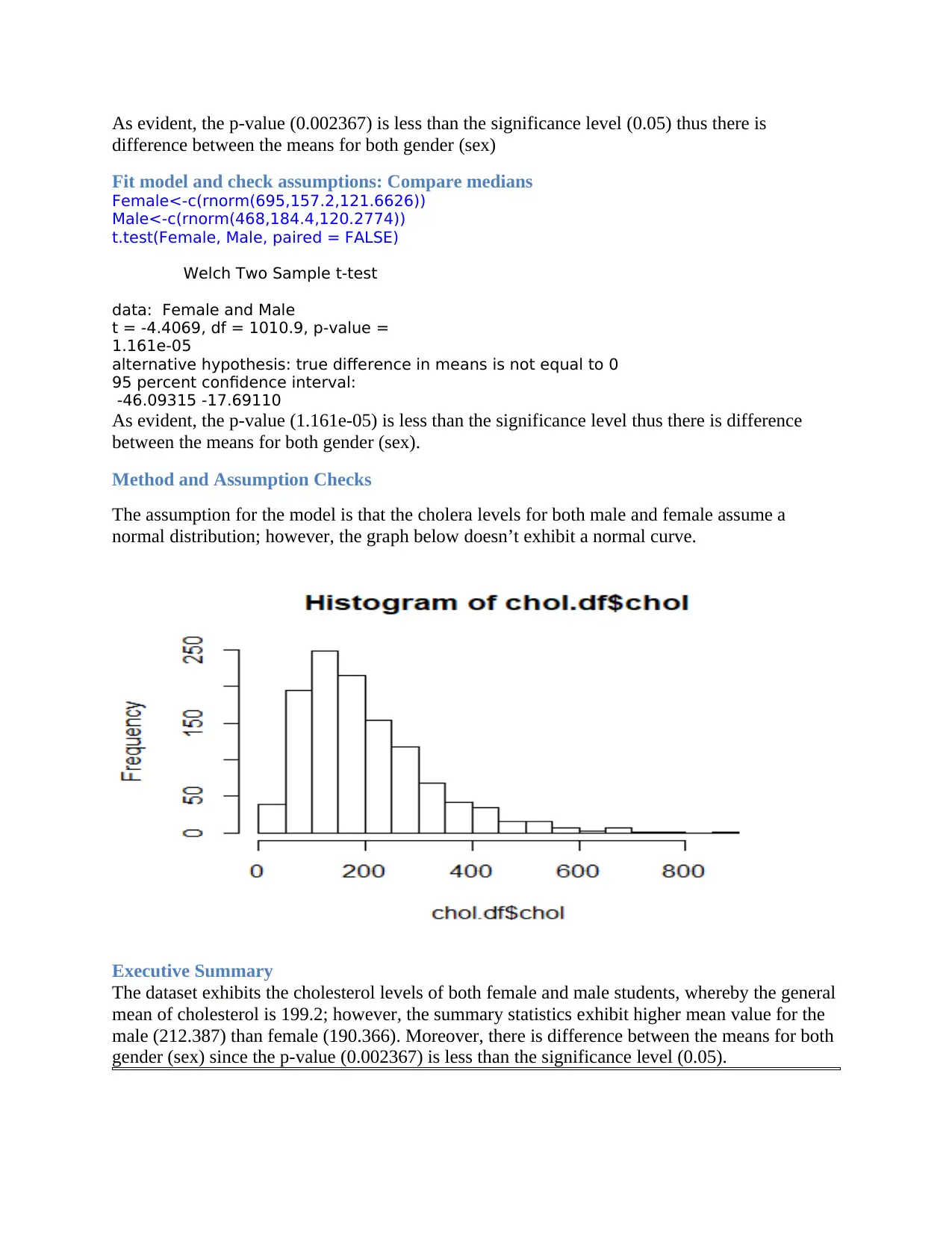
The assumption for the model is that the cholera levels for both male and female assume a
normal distribution; however, the graph below doesn’t exhibit a normal curve.
Executive Summary
The dataset exhibits the cholesterol levels of both female and male students, whereby the general
mean of cholesterol is 199.2; however, the summary statistics exhibit higher mean value for the
male (212.387) than female (190.366). Moreover, there is difference between the means for both
gender (sex) since the p-value (0.002367) is less than the significance level (0.05).
difference between the means for both gender (sex)
Fit model and check assumptions: Compare medians
Female<-c(rnorm(695,157.2,121.6626))
Male<-c(rnorm(468,184.4,120.2774))
t.test(Female, Male, paired = FALSE)
Welch Two Sample t-test
data: Female and Male
t = -4.4069, df = 1010.9, p-value =
1.161e-05
alternative hypothesis: true difference in means is not equal to 0
95 percent confidence interval:
-46.09315 -17.69110
As evident, the p-value (1.161e-05) is less than the significance level thus there is difference
between the means for both gender (sex).
Method and Assumption Checks
The assumption for the model is that the cholera levels for both male and female assume a
normal distribution; however, the graph below doesn’t exhibit a normal curve.
Executive Summary
The dataset exhibits the cholesterol levels of both female and male students, whereby the general
mean of cholesterol is 199.2; however, the summary statistics exhibit higher mean value for the
male (212.387) than female (190.366). Moreover, there is difference between the means for both
gender (sex) since the p-value (0.002367) is less than the significance level (0.05).
⊘ This is a preview!⊘
Do you want full access?
Subscribe today to unlock all pages.
Trusted by 1+ million students worldwide
Question 2
Question of interest/goal of the study
We want to check the power relationship between the colour and their price per carat. In
particular, we want want to estimate how much 50% increase in colour score affects the price of
the diamonds.
Read in and inspect the data:
diamonds.df=read.csv("Diamonds.csv")
diamonds.df$logPrice=log(diamonds.df$Price)
diamonds.df$logColour=log(diamonds.df$Colour)
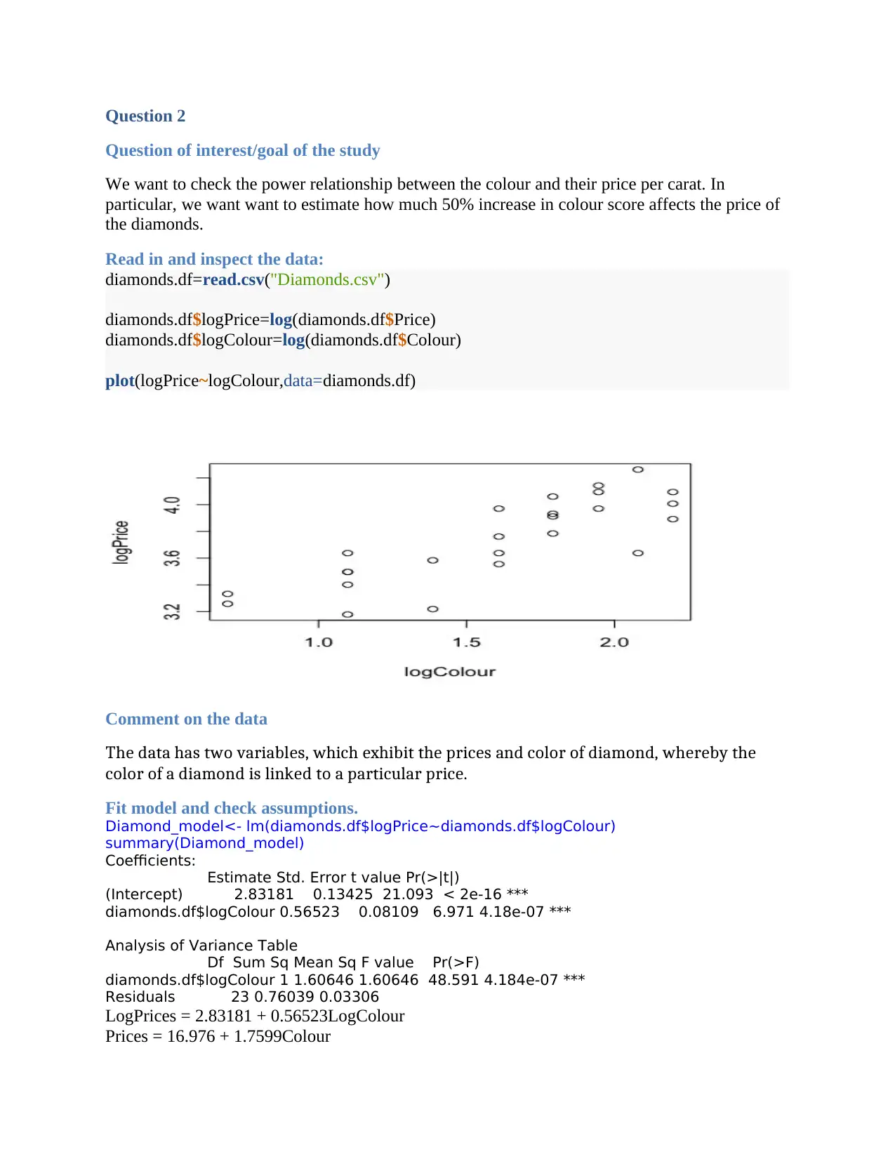
plot(logPrice~logColour,data=diamonds.df)
Comment on the data
The data has two variables, which exhibit the prices and color of diamond, whereby the
color of a diamond is linked to a particular price.
Fit model and check assumptions.
Diamond_model<- lm(diamonds.df$logPrice~diamonds.df$logColour)
summary(Diamond_model)
Coefficients:
Estimate Std. Error t value Pr(>|t|)
(Intercept) 2.83181 0.13425 21.093 < 2e-16 ***
diamonds.df$logColour 0.56523 0.08109 6.971 4.18e-07 ***
Analysis of Variance Table
Df Sum Sq Mean Sq F value Pr(>F)
diamonds.df$logColour 1 1.60646 1.60646 48.591 4.184e-07 ***
Residuals 23 0.76039 0.03306
LogPrices = 2.83181 + 0.56523LogColour
Prices = 16.976 + 1.7599Colour
Question of interest/goal of the study
We want to check the power relationship between the colour and their price per carat. In
particular, we want want to estimate how much 50% increase in colour score affects the price of
the diamonds.
Read in and inspect the data:
diamonds.df=read.csv("Diamonds.csv")
diamonds.df$logPrice=log(diamonds.df$Price)
diamonds.df$logColour=log(diamonds.df$Colour)
plot(logPrice~logColour,data=diamonds.df)
Comment on the data
The data has two variables, which exhibit the prices and color of diamond, whereby the
color of a diamond is linked to a particular price.
Fit model and check assumptions.
Diamond_model<- lm(diamonds.df$logPrice~diamonds.df$logColour)
summary(Diamond_model)
Coefficients:
Estimate Std. Error t value Pr(>|t|)
(Intercept) 2.83181 0.13425 21.093 < 2e-16 ***
diamonds.df$logColour 0.56523 0.08109 6.971 4.18e-07 ***
Analysis of Variance Table
Df Sum Sq Mean Sq F value Pr(>F)
diamonds.df$logColour 1 1.60646 1.60646 48.591 4.184e-07 ***
Residuals 23 0.76039 0.03306
LogPrices = 2.83181 + 0.56523LogColour
Prices = 16.976 + 1.7599Colour
Paraphrase This Document
Need a fresh take? Get an instant paraphrase of this document with our AI Paraphraser
Method and Assumption Checks
The above model exhibits the simple linear regression model, whereby the p-value (<2e-16) is
less than the significance level 0.05 thus showing the model is adequate. There are various
assumption of the model, which include linearity, normality of residuals, homoscedasticity, and
independence of residuals.
plot(Diamond_model)
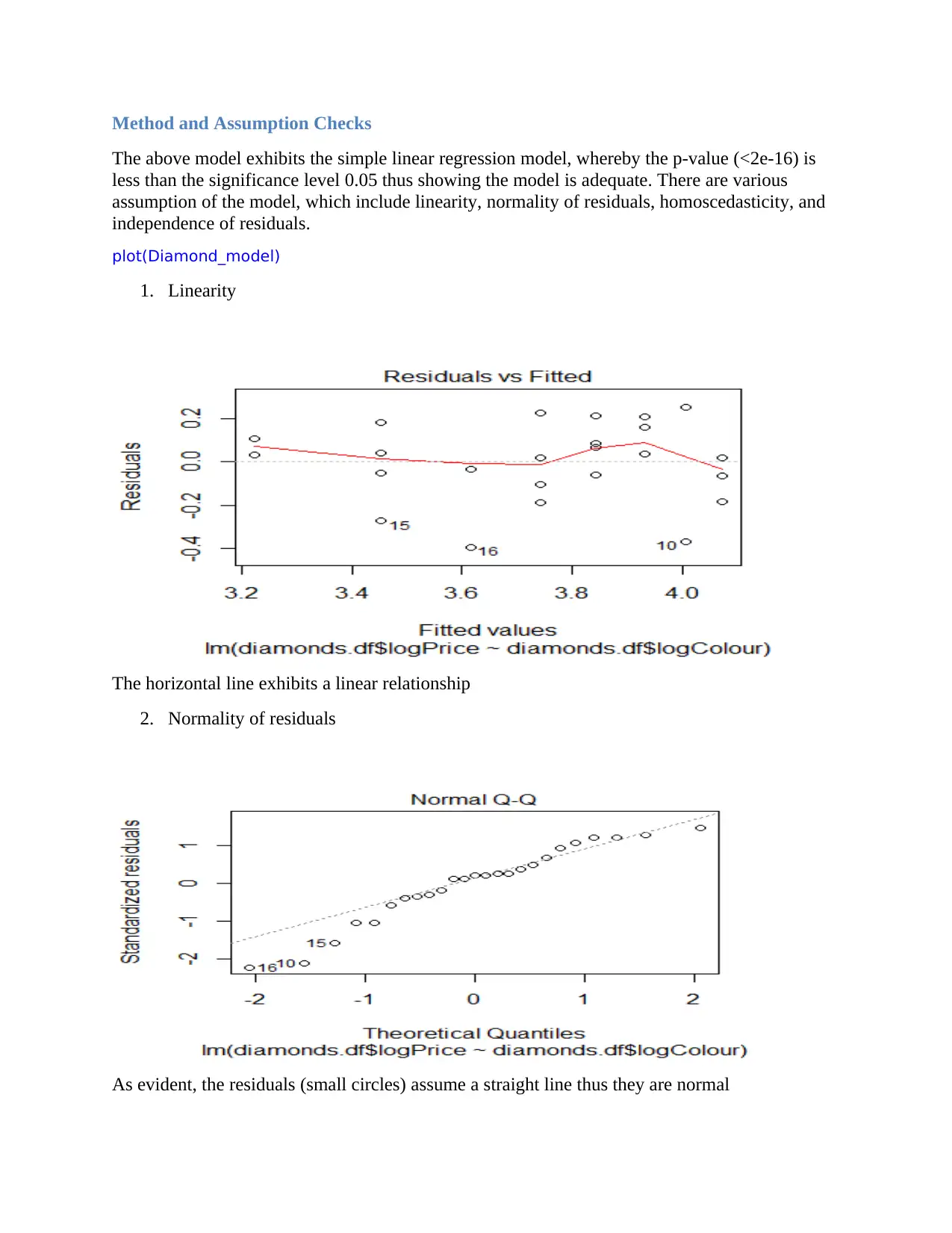
1. Linearity
The horizontal line exhibits a linear relationship
2. Normality of residuals
As evident, the residuals (small circles) assume a straight line thus they are normal
The above model exhibits the simple linear regression model, whereby the p-value (<2e-16) is
less than the significance level 0.05 thus showing the model is adequate. There are various
assumption of the model, which include linearity, normality of residuals, homoscedasticity, and
independence of residuals.
plot(Diamond_model)
1. Linearity
The horizontal line exhibits a linear relationship
2. Normality of residuals
As evident, the residuals (small circles) assume a straight line thus they are normal
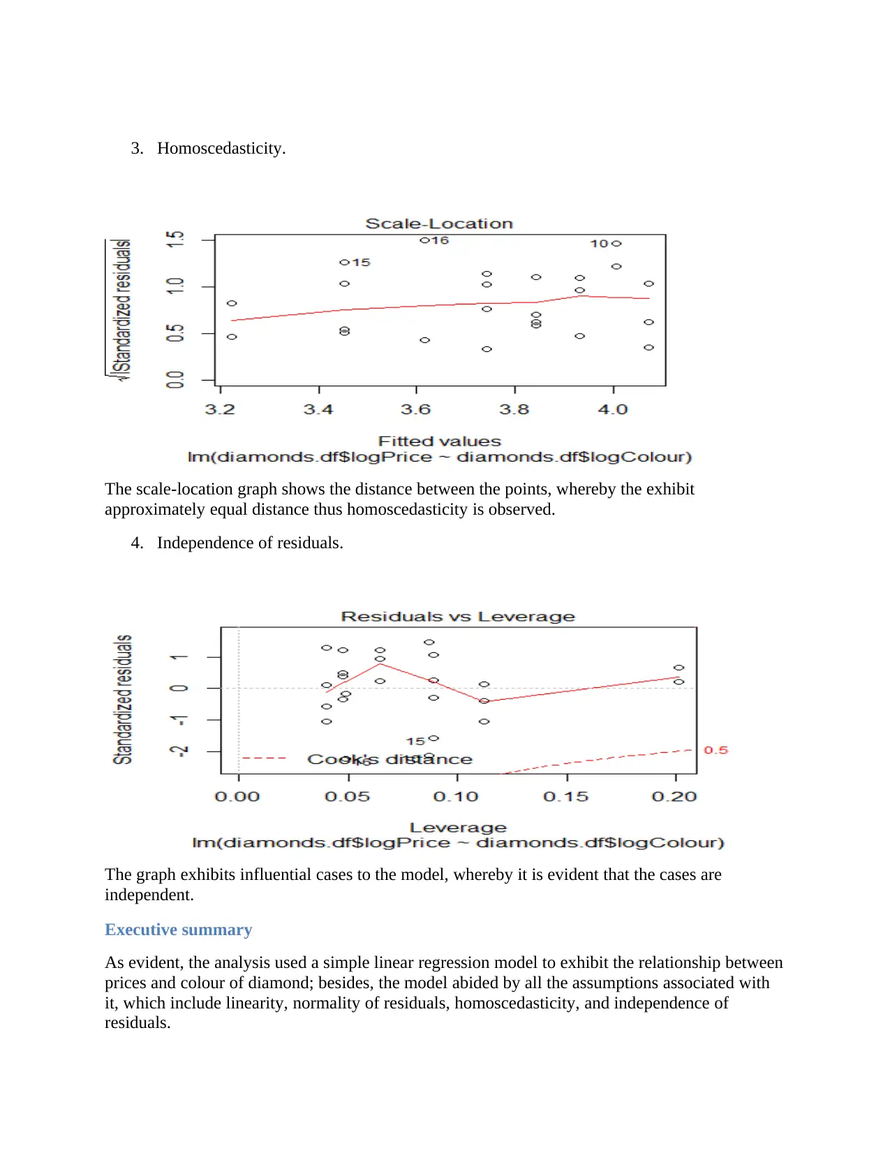
3. Homoscedasticity.
The scale-location graph shows the distance between the points, whereby the exhibit
approximately equal distance thus homoscedasticity is observed.
4. Independence of residuals.
The graph exhibits influential cases to the model, whereby it is evident that the cases are
independent.
Executive summary
As evident, the analysis used a simple linear regression model to exhibit the relationship between
prices and colour of diamond; besides, the model abided by all the assumptions associated with
it, which include linearity, normality of residuals, homoscedasticity, and independence of
residuals.
⊘ This is a preview!⊘
Do you want full access?
Subscribe today to unlock all pages.
Trusted by 1+ million students worldwide
Question 3
Question of interest/goal of the study
We are interested in whether FDG scores are different between normal individuals and AD
patients. If there is a difference, does this difference depends on age?
Read in and inspect the data:
adni.df=read.table("ADNI.txt",header=T)
color=rep('black',nrow(adni.df))
color[adni.df$Status=="AD"]="blue"
color[adni.df$Status=="CN"]="red"
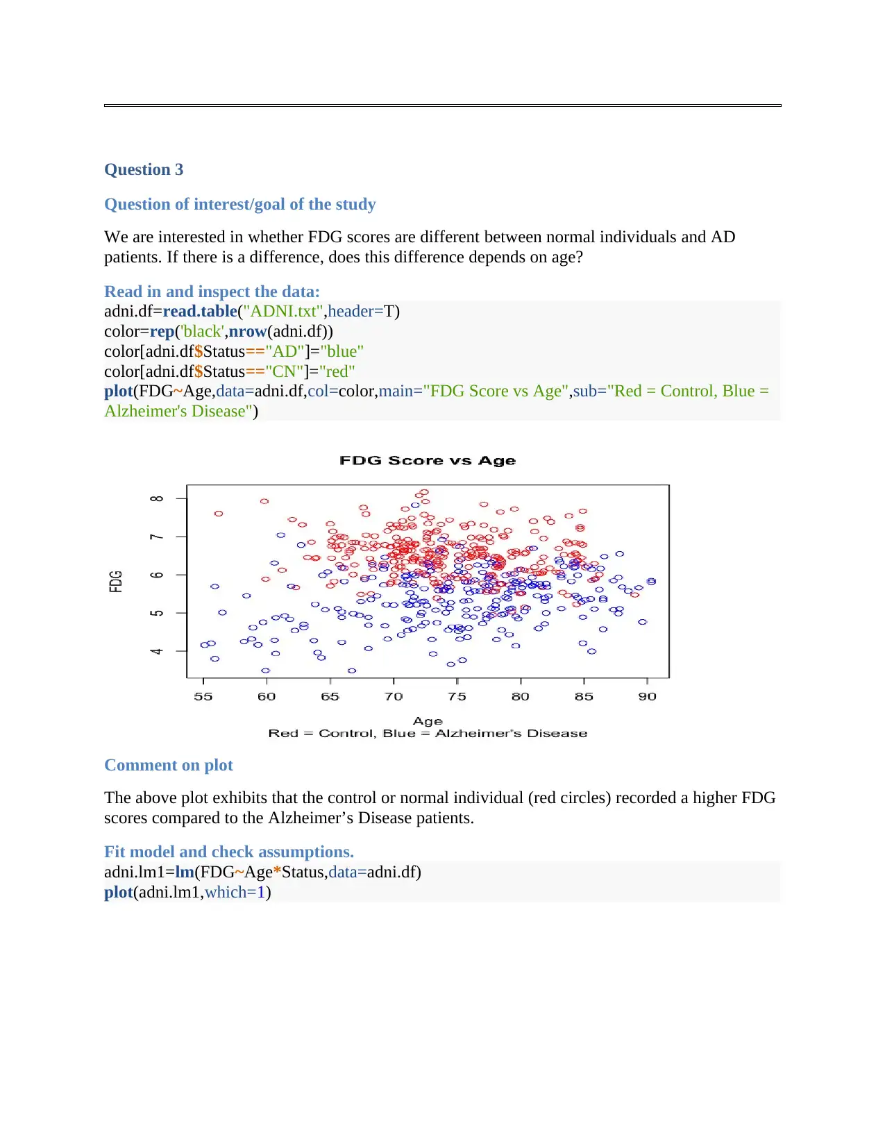
plot(FDG~Age,data=adni.df,col=color,main="FDG Score vs Age",sub="Red = Control, Blue =
Alzheimer's Disease")
Comment on plot
The above plot exhibits that the control or normal individual (red circles) recorded a higher FDG
scores compared to the Alzheimer’s Disease patients.
Fit model and check assumptions.
adni.lm1=lm(FDG~Age*Status,data=adni.df)
plot(adni.lm1,which=1)
Question of interest/goal of the study
We are interested in whether FDG scores are different between normal individuals and AD
patients. If there is a difference, does this difference depends on age?
Read in and inspect the data:
adni.df=read.table("ADNI.txt",header=T)
color=rep('black',nrow(adni.df))
color[adni.df$Status=="AD"]="blue"
color[adni.df$Status=="CN"]="red"
plot(FDG~Age,data=adni.df,col=color,main="FDG Score vs Age",sub="Red = Control, Blue =
Alzheimer's Disease")
Comment on plot
The above plot exhibits that the control or normal individual (red circles) recorded a higher FDG
scores compared to the Alzheimer’s Disease patients.
Fit model and check assumptions.
adni.lm1=lm(FDG~Age*Status,data=adni.df)
plot(adni.lm1,which=1)
Paraphrase This Document
Need a fresh take? Get an instant paraphrase of this document with our AI Paraphraser
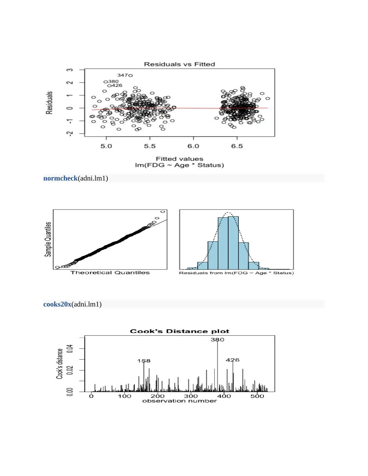
normcheck(adni.lm1)
cooks20x(adni.lm1)
cooks20x(adni.lm1)
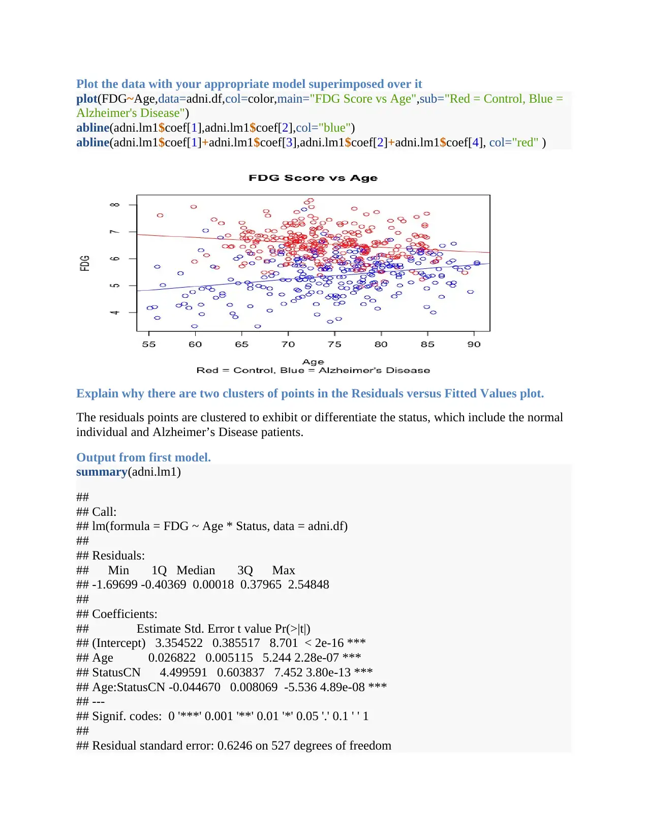
Plot the data with your appropriate model superimposed over it
plot(FDG~Age,data=adni.df,col=color,main="FDG Score vs Age",sub="Red = Control, Blue =
Alzheimer's Disease")
abline(adni.lm1$coef[1],adni.lm1$coef[2],col="blue")
abline(adni.lm1$coef[1]+adni.lm1$coef[3],adni.lm1$coef[2]+adni.lm1$coef[4], col="red" )
Explain why there are two clusters of points in the Residuals versus Fitted Values plot.
The residuals points are clustered to exhibit or differentiate the status, which include the normal
individual and Alzheimer’s Disease patients.
Output from first model.
summary(adni.lm1)
##
## Call:
## lm(formula = FDG ~ Age * Status, data = adni.df)
##
## Residuals:
## Min 1Q Median 3Q Max
## -1.69699 -0.40369 0.00018 0.37965 2.54848
##
## Coefficients:
## Estimate Std. Error t value Pr(>|t|)
## (Intercept) 3.354522 0.385517 8.701 < 2e-16 ***
## Age 0.026822 0.005115 5.244 2.28e-07 ***
## StatusCN 4.499591 0.603837 7.452 3.80e-13 ***
## Age:StatusCN -0.044670 0.008069 -5.536 4.89e-08 ***
## ---
## Signif. codes: 0 '***' 0.001 '**' 0.01 '*' 0.05 '.' 0.1 ' ' 1
##
## Residual standard error: 0.6246 on 527 degrees of freedom
⊘ This is a preview!⊘
Do you want full access?
Subscribe today to unlock all pages.
Trusted by 1+ million students worldwide
## Multiple R-squared: 0.4836, Adjusted R-squared: 0.4806
## F-statistic: 164.5 on 3 and 527 DF, p-value: < 2.2e-16
confint(adni.lm1)
## 2.5 % 97.5 %
## (Intercept) 2.59718306 4.11186155
## Age 0.01677362 0.03687132
## StatusCN 3.31336858 5.68581315
## Age:StatusCN -0.06052069 -0.02881862
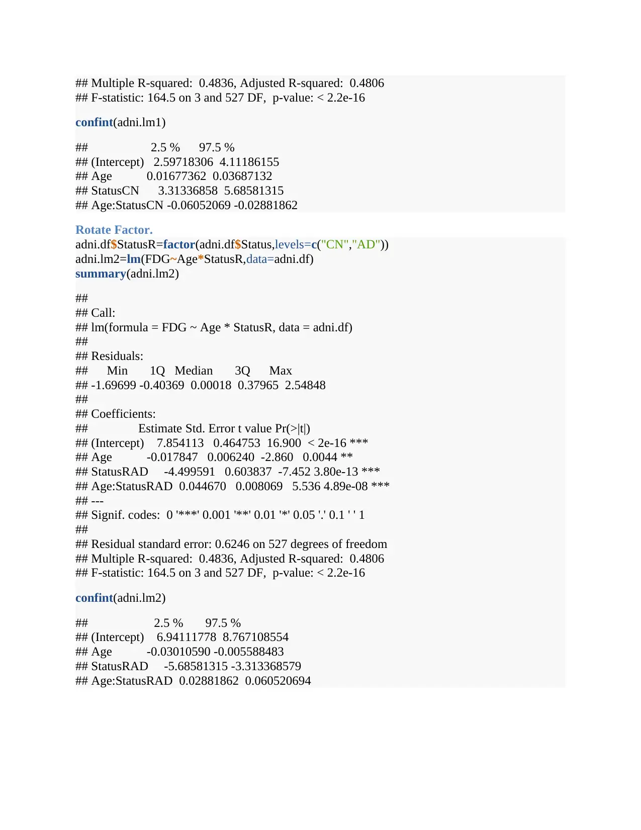
Rotate Factor.
adni.df$StatusR=factor(adni.df$Status,levels=c("CN","AD"))
adni.lm2=lm(FDG~Age*StatusR,data=adni.df)
summary(adni.lm2)
##
## Call:
## lm(formula = FDG ~ Age * StatusR, data = adni.df)
##
## Residuals:
## Min 1Q Median 3Q Max
## -1.69699 -0.40369 0.00018 0.37965 2.54848
##
## Coefficients:
## Estimate Std. Error t value Pr(>|t|)
## (Intercept) 7.854113 0.464753 16.900 < 2e-16 ***
## Age -0.017847 0.006240 -2.860 0.0044 **
## StatusRAD -4.499591 0.603837 -7.452 3.80e-13 ***
## Age:StatusRAD 0.044670 0.008069 5.536 4.89e-08 ***
## ---
## Signif. codes: 0 '***' 0.001 '**' 0.01 '*' 0.05 '.' 0.1 ' ' 1
##
## Residual standard error: 0.6246 on 527 degrees of freedom
## Multiple R-squared: 0.4836, Adjusted R-squared: 0.4806
## F-statistic: 164.5 on 3 and 527 DF, p-value: < 2.2e-16
confint(adni.lm2)
## 2.5 % 97.5 %
## (Intercept) 6.94111778 8.767108554
## Age -0.03010590 -0.005588483
## StatusRAD -5.68581315 -3.313368579
## Age:StatusRAD 0.02881862 0.060520694
## F-statistic: 164.5 on 3 and 527 DF, p-value: < 2.2e-16
confint(adni.lm1)
## 2.5 % 97.5 %
## (Intercept) 2.59718306 4.11186155
## Age 0.01677362 0.03687132
## StatusCN 3.31336858 5.68581315
## Age:StatusCN -0.06052069 -0.02881862
Rotate Factor.
adni.df$StatusR=factor(adni.df$Status,levels=c("CN","AD"))
adni.lm2=lm(FDG~Age*StatusR,data=adni.df)
summary(adni.lm2)
##
## Call:
## lm(formula = FDG ~ Age * StatusR, data = adni.df)
##
## Residuals:
## Min 1Q Median 3Q Max
## -1.69699 -0.40369 0.00018 0.37965 2.54848
##
## Coefficients:
## Estimate Std. Error t value Pr(>|t|)
## (Intercept) 7.854113 0.464753 16.900 < 2e-16 ***
## Age -0.017847 0.006240 -2.860 0.0044 **
## StatusRAD -4.499591 0.603837 -7.452 3.80e-13 ***
## Age:StatusRAD 0.044670 0.008069 5.536 4.89e-08 ***
## ---
## Signif. codes: 0 '***' 0.001 '**' 0.01 '*' 0.05 '.' 0.1 ' ' 1
##
## Residual standard error: 0.6246 on 527 degrees of freedom
## Multiple R-squared: 0.4836, Adjusted R-squared: 0.4806
## F-statistic: 164.5 on 3 and 527 DF, p-value: < 2.2e-16
confint(adni.lm2)
## 2.5 % 97.5 %
## (Intercept) 6.94111778 8.767108554
## Age -0.03010590 -0.005588483
## StatusRAD -5.68581315 -3.313368579
## Age:StatusRAD 0.02881862 0.060520694
Paraphrase This Document
Need a fresh take? Get an instant paraphrase of this document with our AI Paraphraser

Method and Assumption Checks
As evident, the Q-Q and histogram plots exhibits a normal distribution thus the residual
assume normal distribution. Moreover, the cooks distance plot shows the independence in
the residuals.
In terms of slopes and/or intercepts, explain what the coefficient of Age:StatusCN is
estimating.
As exhibited, the coefficient of Age:StatusCN is -0.044670, which indicates the interaction
between the age and CN reduces the FDG scores by 0.044670.
For each of the following, either write a sentence interpreting a confidence interval to
estimate the requested information or state why we cannot answer this from the R-output
given:
- in general, the difference in size of FDG scores between healthy people and those with
Alzheimer’s disease.
The R-output does not provide sufficient evidence to show the difference thus it cannot be used,
- the effect on the FDG scores for each additional years aging on healthy people.
The coefficient of age associated with healthy people is 0.026822 thus, for any additional year of
a healthy person the FDG scores increases by 0.026822.
- the effect on the FDG scores for each additional years aging on people with Alzheimer’s
disease.
The coefficient of age associated with healthy people is -0.017847 thus, for any additional year
of Alzheimer disease patient the FDG scores increases by 0.017847.
Looking at the plot with the model superimposed, describe what seems to be happening.
The plot shows for the Alzheimer disease the FDG scores increases with age whereas for healthy
people FDG scores reduces with age.
Plot prediction intervals for FDG scores verses age ranges for the two groups
plot(FDG~Age,data=adni.df,main="Prediction Intervals for FDG Score vs Age",sub="Red =
Control, Blue = Alzheimer's Disease",type="n")
abline(adni.lm1$coef[1],adni.lm1$coef[2],col="blue")
abline(adni.lm1$coef[1]+adni.lm1$coef[3],adni.lm1$coef[2]+adni.lm1$coef[4], col="red" )
ages=seq(55,90,by=0.1)
predAD=as.factor(rep("AD",length(ages)))
predCN=as.factor(rep("CN",length(ages)))
new.dat1=data.frame(Age=ages, Status=predAD)
new.dat2=data.frame(Age=ages, Status=predCN)
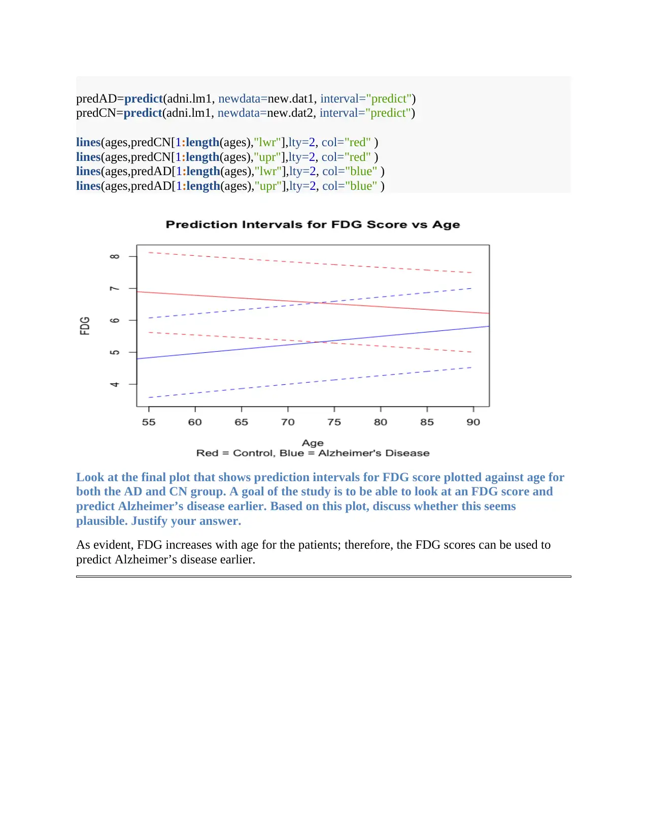
predAD=predict(adni.lm1, newdata=new.dat1, interval="predict")
predCN=predict(adni.lm1, newdata=new.dat2, interval="predict")
lines(ages,predCN[1:length(ages),"lwr"],lty=2, col="red" )
lines(ages,predCN[1:length(ages),"upr"],lty=2, col="red" )
lines(ages,predAD[1:length(ages),"lwr"],lty=2, col="blue" )
lines(ages,predAD[1:length(ages),"upr"],lty=2, col="blue" )
Look at the final plot that shows prediction intervals for FDG score plotted against age for
both the AD and CN group. A goal of the study is to be able to look at an FDG score and
predict Alzheimer’s disease earlier. Based on this plot, discuss whether this seems
plausible. Justify your answer.
As evident, FDG increases with age for the patients; therefore, the FDG scores can be used to
predict Alzheimer’s disease earlier.
⊘ This is a preview!⊘
Do you want full access?
Subscribe today to unlock all pages.
Trusted by 1+ million students worldwide
1 out of 12
Related Documents


Your All-in-One AI-Powered Toolkit for Academic Success.
+13062052269
info@desklib.com
Available 24*7 on WhatsApp / Email
![[object Object]](/_next/static/media/star-bottom.7253800d.svg)
Unlock your academic potential
Copyright © 2020–2026 A2Z Services. All Rights Reserved. Developed and managed by ZUCOL.