ECON 2330: Group Assignment III - Regression, Trendlines, and Analysis

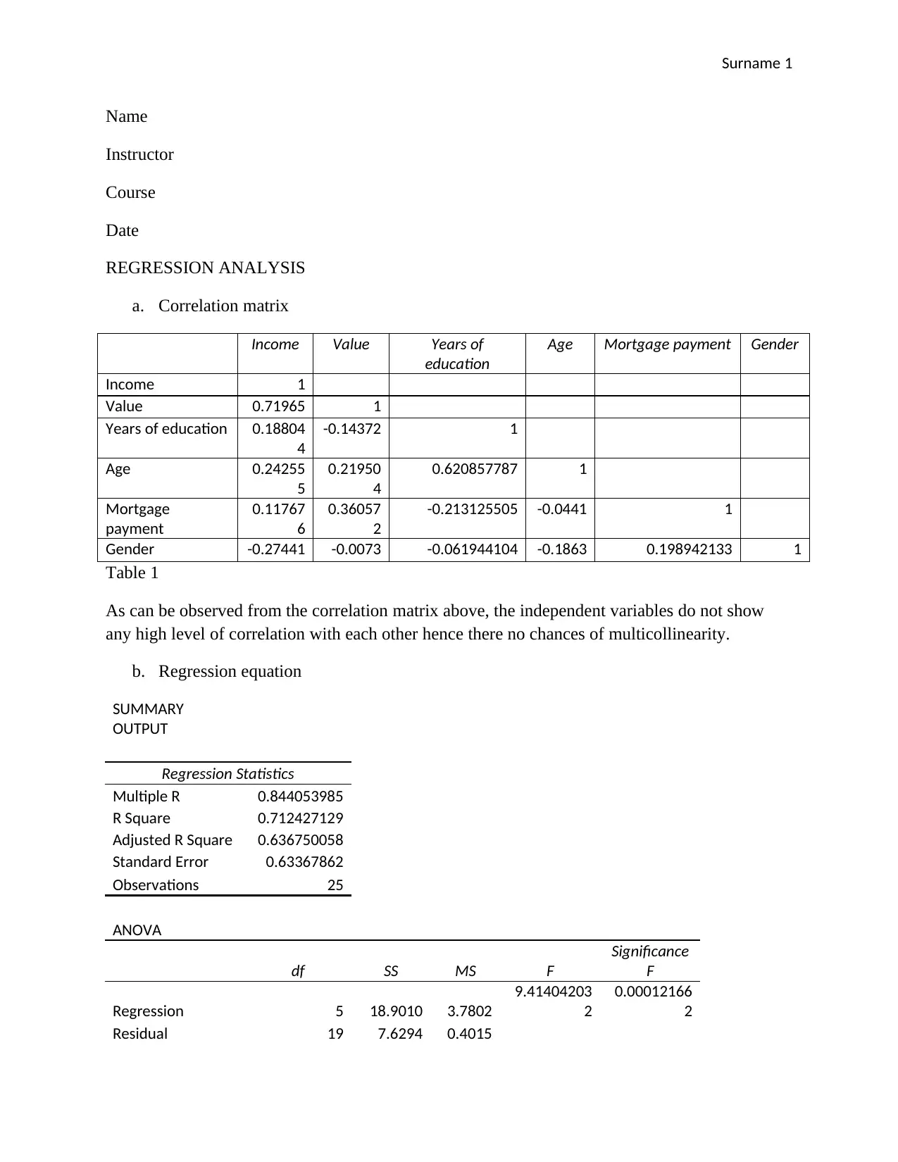
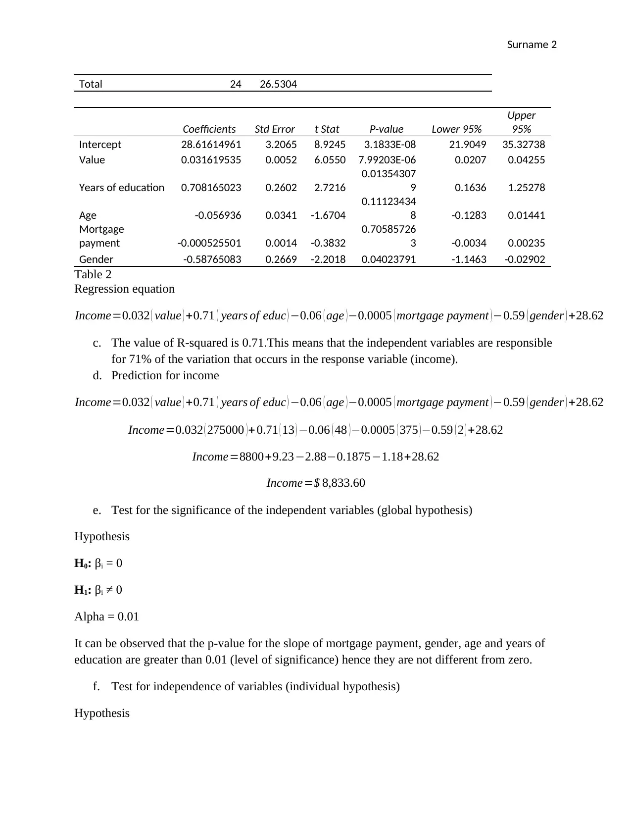
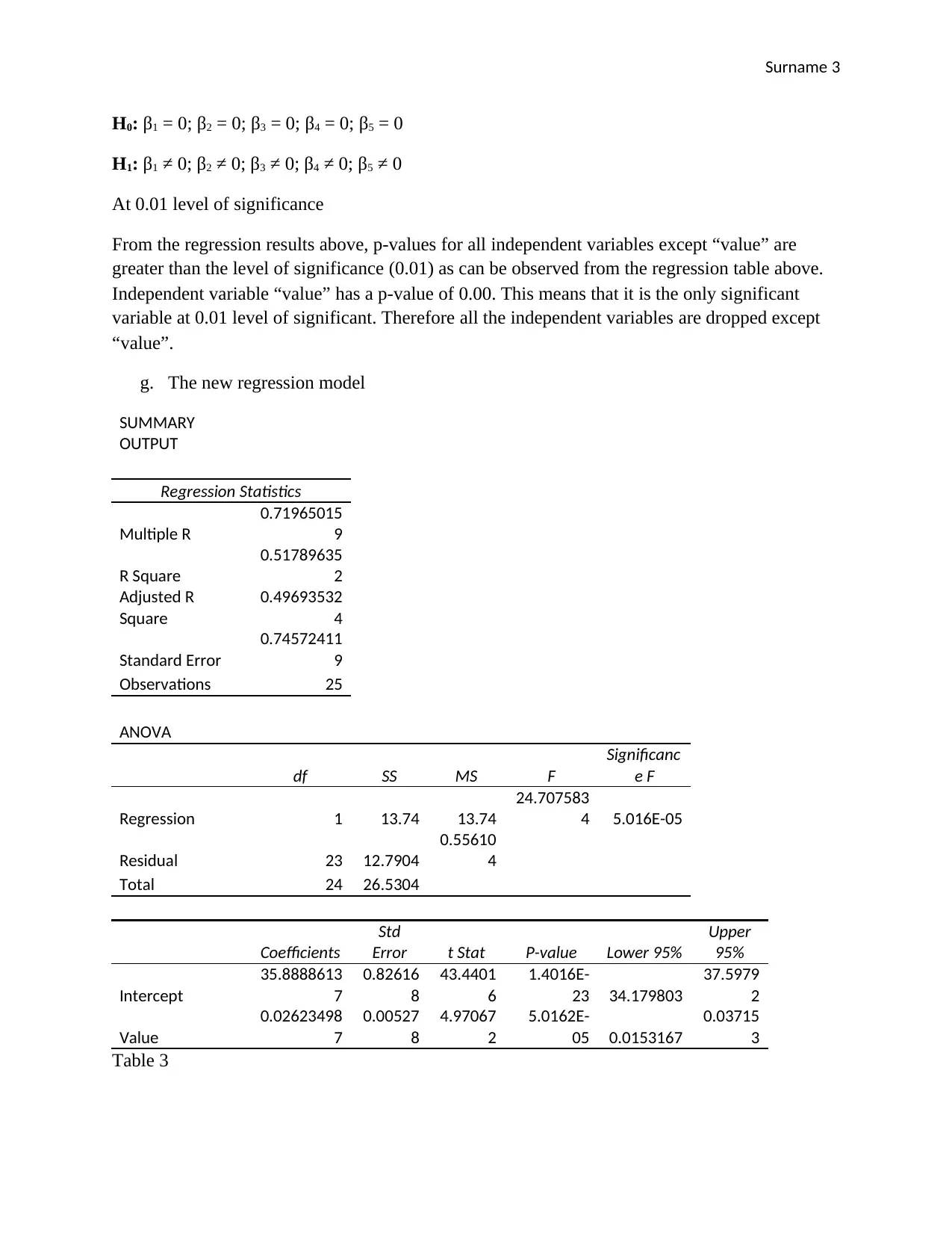
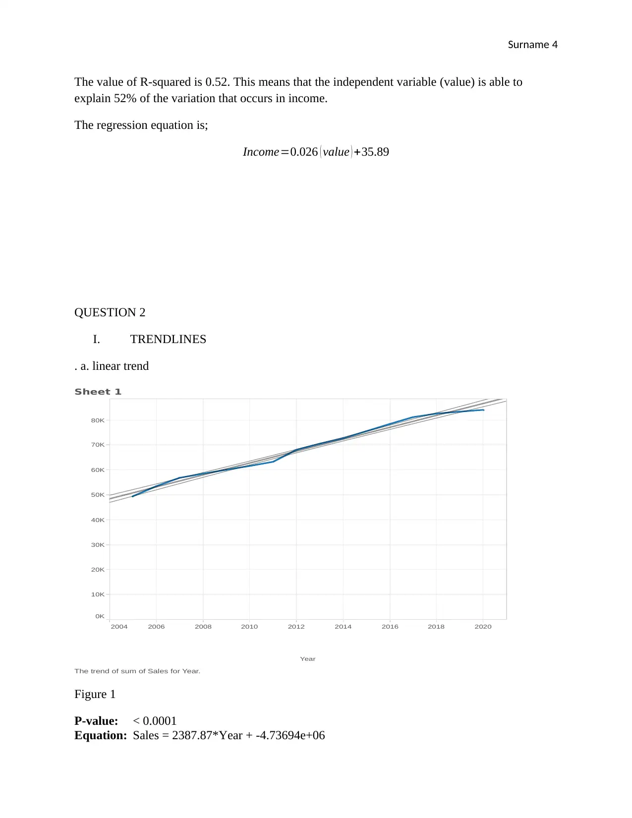
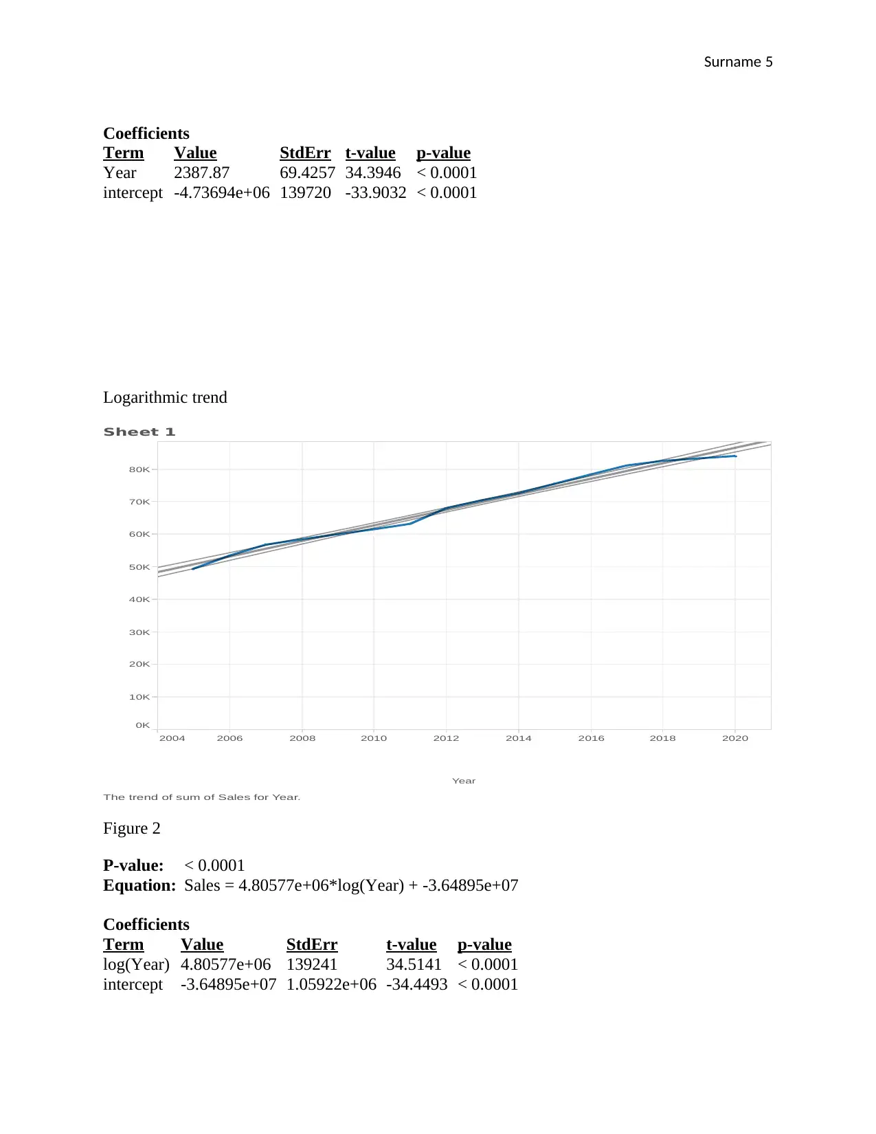
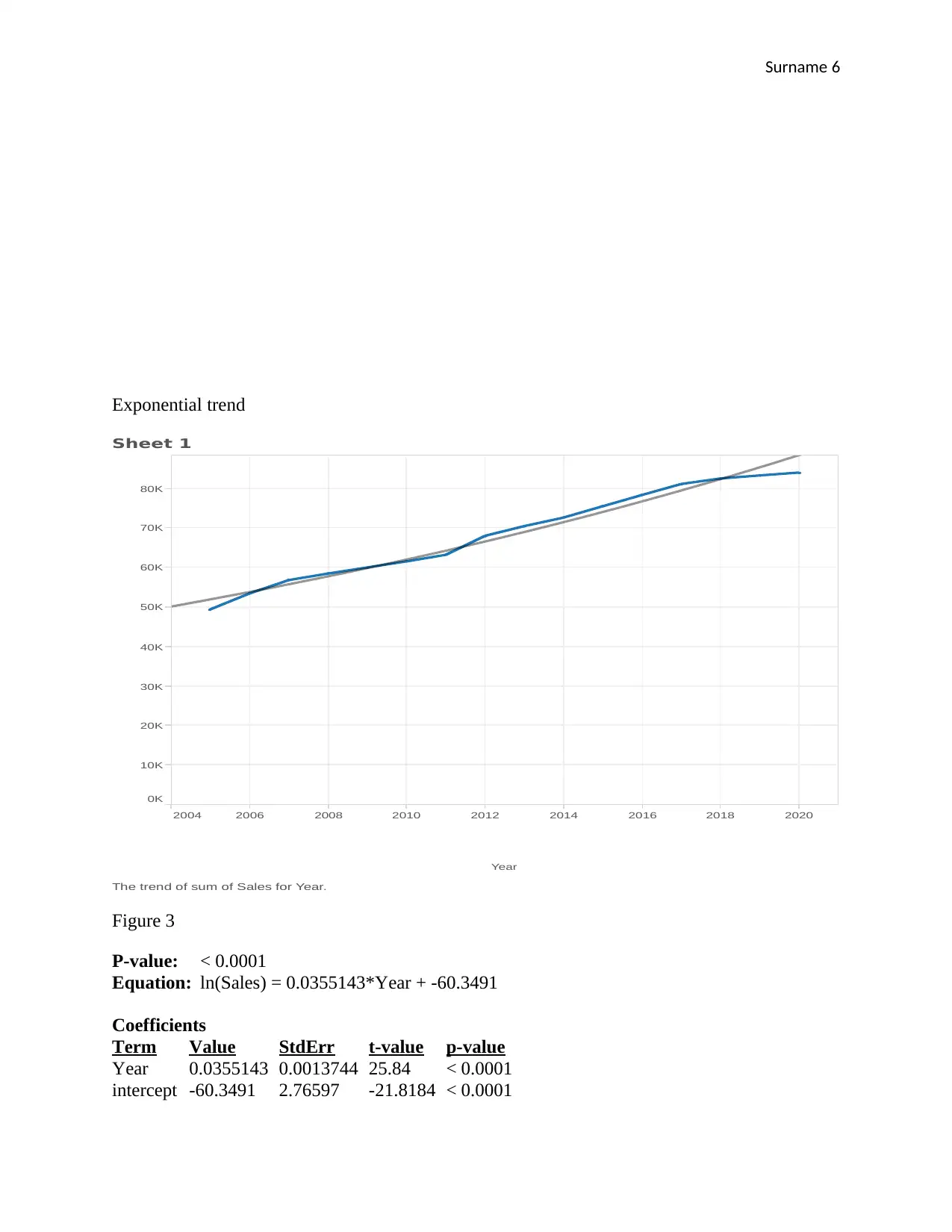
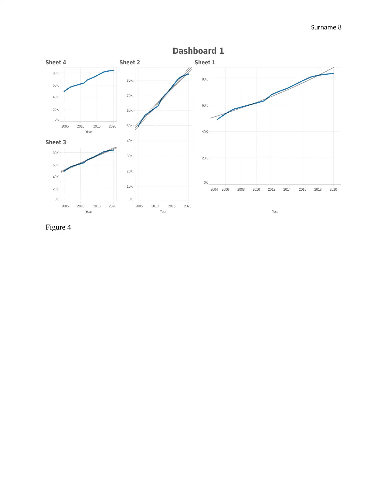
This document presents a comprehensive solution to an ECON 2330 group assignment. The assignment focuses on regression analysis, exploring the relationship between income and various factors like home value, education, age, mortgage payments, and gender. The solution includes the development of a correlation matrix to assess multicollinearity, the determination of the regression equation, interpretation of R-squared, and prediction of income based on given characteristics. Furthermore, the assignment delves into trendline analysis, comparing linear, logarithmic, and exponential trends to forecast sales. The analysis includes p-values, equations, and R-squared values for each trendline, culminating in a recommendation for the most suitable trendline and a 2022 sales estimate. The document also provides a summary of sales data and a dashboard visualization, demonstrating a thorough understanding of statistical analysis and forecasting techniques.

Surname 1
Name
Instructor
Course
Date
REGRESSION ANALYSIS
a. Correlation matrix
Income Value Years of
education
Age Mortgage payment Gender
Income 1
Value 0.71965 1
Years of education 0.18804
4
-0.14372 1
Age 0.24255
5
0.21950
4
0.620857787 1
Mortgage
payment
0.11767
6
0.36057
2
-0.213125505 -0.0441 1
Gender -0.27441 -0.0073 -0.061944104 -0.1863 0.198942133 1
Table 1
As can be observed from the correlation matrix above, the independent variables do not show
any high level of correlation with each other hence there no chances of multicollinearity.
b. Regression equation
SUMMARY
OUTPUT
Regression Statistics
Multiple R 0.844053985
R Square 0.712427129
Adjusted R Square 0.636750058
Standard Error 0.63367862
Observations 25
ANOVA
df SS MS F
Significance
F
Regression 5 18.9010 3.7802
9.41404203
2
0.00012166
2
Residual 19 7.6294 0.4015

Surname 2
Total 24 26.5304
Coefficients Std Error t Stat P-value Lower 95%
Upper
95%
Intercept 28.61614961 3.2065 8.9245 3.1833E-08 21.9049 35.32738
Value 0.031619535 0.0052 6.0550 7.99203E-06 0.0207 0.04255
Years of education 0.708165023 0.2602 2.7216
0.01354307
9 0.1636 1.25278
Age -0.056936 0.0341 -1.6704
0.11123434
8 -0.1283 0.01441
Mortgage
payment -0.000525501 0.0014 -0.3832
0.70585726
3 -0.0034 0.00235
Gender -0.58765083 0.2669 -2.2018 0.04023791 -1.1463 -0.02902
Table 2
Regression equation
Income=0.032 ( value ) +0.71 ( years of educ ) −0.06 ( age )−0.0005 ( mortgage payment )−0.59 ( gender ) +28.62
c. The value of R-squared is 0.71.This means that the independent variables are responsible
for 71% of the variation that occurs in the response variable (income).
d. Prediction for income
Income=0.032 ( value ) +0.71 ( years of educ ) −0.06 ( age )−0.0005 ( mortgage payment )−0.59 ( gender ) +28.62
Income=0.032 ( 275000 )+ 0.71 ( 13 ) −0.06 ( 48 )−0.0005 ( 375 )−0.59 ( 2 ) +28.62
Income=8800+9.23−2.88−0.1875−1.18+28.62
Income=$ 8,833.60
e. Test for the significance of the independent variables (global hypothesis)
Hypothesis
H0: βi = 0
H1: βi ≠ 0
Alpha = 0.01
It can be observed that the p-value for the slope of mortgage payment, gender, age and years of
education are greater than 0.01 (level of significance) hence they are not different from zero.
f. Test for independence of variables (individual hypothesis)
Hypothesis

Surname 3
H0: β1 = 0; β2 = 0; β3 = 0; β4 = 0; β5 = 0
H1: β1 ≠ 0; β2 ≠ 0; β3 ≠ 0; β4 ≠ 0; β5 ≠ 0
At 0.01 level of significance
From the regression results above, p-values for all independent variables except “value” are
greater than the level of significance (0.01) as can be observed from the regression table above.
Independent variable “value” has a p-value of 0.00. This means that it is the only significant
variable at 0.01 level of significant. Therefore all the independent variables are dropped except
“value”.
g. The new regression model
SUMMARY
OUTPUT
Regression Statistics
Multiple R
0.71965015
9
R Square
0.51789635
2
Adjusted R
Square
0.49693532
4
Standard Error
0.74572411
9
Observations 25
ANOVA
df SS MS F
Significanc
e F
Regression 1 13.74 13.74
24.707583
4 5.016E-05
Residual 23 12.7904
0.55610
4
Total 24 26.5304
Coefficients
Std
Error t Stat P-value Lower 95%
Upper
95%
Intercept
35.8888613
7
0.82616
8
43.4401
6
1.4016E-
23 34.179803
37.5979
2
Value
0.02623498
7
0.00527
8
4.97067
2
5.0162E-
05 0.0153167
0.03715
3
Table 3

Surname 4
The value of R-squared is 0.52. This means that the independent variable (value) is able to
explain 52% of the variation that occurs in income.
The regression equation is;
Income=0.026 ( value ) +35.89
QUESTION 2
I. TRENDLINES
. a. linear trend
2004 2006 2008 2010 2012 2014 2016 2018 2020
Year
0K
10K
20K
30K
40K
50K
60K
70K
80K
Sales
Sheet 1
The trend of sum of Sales for Year.
Figure 1
P-value: < 0.0001
Equation: Sales = 2387.87*Year + -4.73694e+06

Surname 5
Coefficients
Term Value StdErr t-value p-value
Year 2387.87 69.4257 34.3946 < 0.0001
intercept -4.73694e+06 139720 -33.9032 < 0.0001
Logarithmic trend
2004 2006 2008 2010 2012 2014 2016 2018 2020
Year
0K
10K
20K
30K
40K
50K
60K
70K
80K
Sales
Sheet 1
The trend of sum of Sales for Year.
Figure 2
P-value: < 0.0001
Equation: Sales = 4.80577e+06*log(Year) + -3.64895e+07
Coefficients
Term Value StdErr t-value p-value
log(Year) 4.80577e+06 139241 34.5141 < 0.0001
intercept -3.64895e+07 1.05922e+06 -34.4493 < 0.0001

Surname 6
Exponential trend
2004 2006 2008 2010 2012 2014 2016 2018 2020
Year
0K
10K
20K
30K
40K
50K
60K
70K
80K
Sales
Sheet 1
The trend of sum of Sales for Year.
Figure 3
P-value: < 0.0001
Equation: ln(Sales) = 0.0355143*Year + -60.3491
Coefficients
Term Value StdErr t-value p-value
Year 0.0355143 0.0013744 25.84 < 0.0001
intercept -60.3491 2.76597 -21.8184 < 0.0001

Surname 7
II. I would suggest linear trendline. This is because it has got a higher R-squared value
(0.988) compared to exponential and logarithmic trend.
III. 2022 sales estimate
Equation: Sales = 2387.87*Year + -4.73694e+06
Sales = 2387.87*2022 + -4.73694e+06
Sales = 4828273.14 – 4736940 = 91,333.14
The sales estimates are very reasonable given the sales for 2020 was about 85,000.
IV. Summary
Count: 16
SUM(Sales)
Sum: 1,098,469
Average: 68,654.31
Minimum: 49,378
Maximum: 84,005
Median: 69,218.50
V. Dashboard

Surname 8
Dashboard 1
2004 2006 2008 2010 2012 2014 2016 2018 2020
Year
0K
20K
40K
60K
80K
Sheet 1
2005 2010 2015 2020
Year
0K
10K
20K
30K
40K
50K
60K
70K
80K
Sheet 2
2005 2010 2015 2020
Year
0K
20K
40K
60K
80K
Sheet 3
2005 2010 2015 2020
Year
0K
20K
40K
60K
80K
Sheet 4
Figure 4