Assessment Task 2: Simple & Multiple Linear Regression Analysis Report

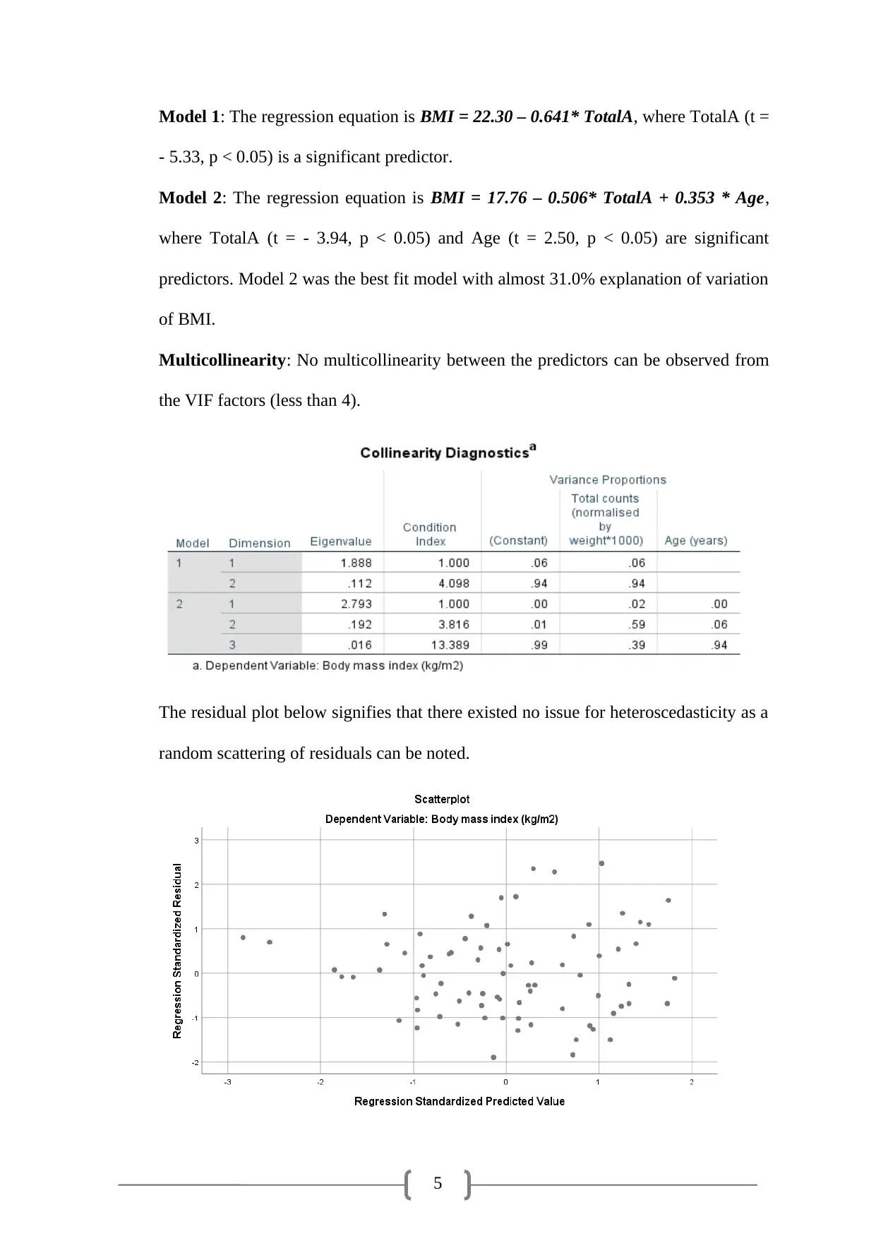
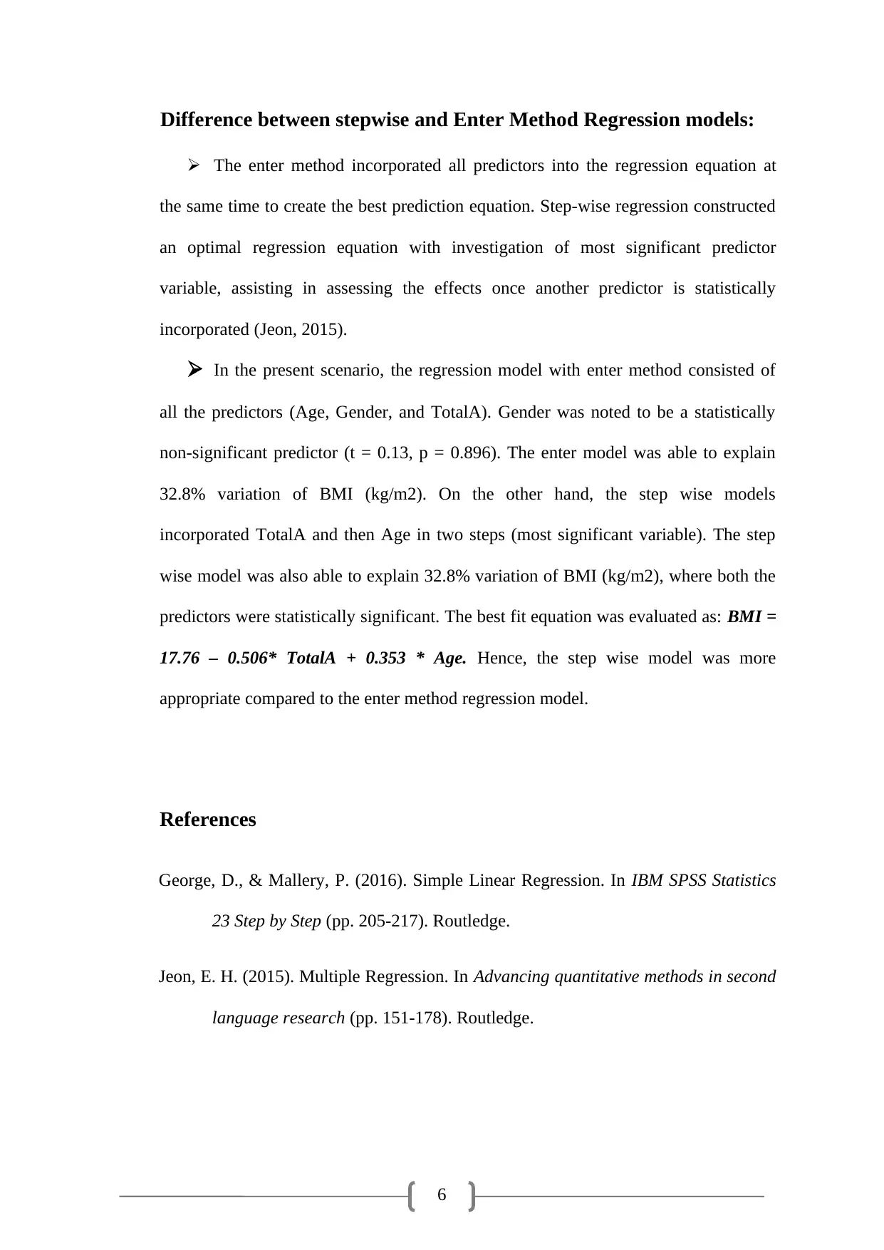
This assignment presents a detailed analysis of simple and multiple linear regression models using statistical techniques. The student conducted a simple linear regression to assess the relationship between total daily activity (TotalA) and Body Mass Index (BMI), finding a negative correlation and explaining 27.2% of the variance in BMI. The analysis then extends to multiple linear regression, comparing stepwise and enter methods. Two models were developed: one with TotalA alone and another with Age and TotalA. The stepwise model incorporated TotalA and then Age, explaining 31.0% of the BMI variation. The enter method, including Age, Gender, and TotalA, explained 32.8% of the variance. The student evaluated the models, highlighting the significance of predictors, multicollinearity, and heteroscedasticity, concluding the stepwise model was more appropriate. The assignment includes regression equations, statistical outputs, and references to relevant literature.

1
Activity 4: Simple & Multiple Linear Regression

2
A. Simple (Bivariate) Linear Regression
Exercise:
1. From the regression output it was noted that total amount of daily activity (TotalA) was
able to explain 27.2% variability in BMI (R2 = 0.272).
2. The regression equation was: BMI (Y) = 22.30 – 0.64 * TotalA (X).
3. BMI and TotalA have a significantly negative, and moderate correlation between them
(r = - 0.52, p < 0.05).
4. The scatterplot between both the variables has been drawn to assess the linear fit and
presence of outliers (George, & Mallery, 2016).
 The scatterplot in above figure reveals a decreasing trend for BMI (kg/m2) for increase
in total amount of daily activity. Hence, a negative correlation can be identified
between the two variables.
 Few major outliers can be noted from the scatterplot (marked red). These BMI scores
are lower/higher than other BMI scores with similar amount of daily activity.

3
 The linear model was appropriate for this data as the residuals in the residual plot was
homogeneously scattered. Hence, the regression line was appropriate fit. The R2 in the
scatterplot between TotalA and BMI revealed that total amount of daily activity was
able to explain BMI (kg/m2).
5. “A linear regression analysis was conducted to evaluate the prediction that” TotalA was
relatively accurate in predicting the BMI. “The correlation between” TotalA and BMI
was – 0.522. Approximately 27.2% of the variance in BMI “was accounted for by its
linear relationship with” TotalA.

4
B. Multiple Linear Regression
Exercise:
Brief Summary of stepwise regression models:
Dependent variable: BMI (kg/m2)
Independent Variables: Age, Gender, TotalA
Model 1: Predictors selected: TotalA
Model 2: Predictors selected: Age and TotalA
Bivariate correlation between TotalA and BMI was moderately negative, but
statistically significant (r = -0.522, p < 0.05). TotalA was able to explain almost
27.2% variation of BMI. In model 2, overall correlation was significant (r = 0.573, p
< 0.05) where Age and TotalA were able to explain almost 31.0% variation of BMI.

5
Model 1: The regression equation is BMI = 22.30 – 0.641* TotalA, where TotalA (t =
- 5.33, p < 0.05) is a significant predictor.
Model 2: The regression equation is BMI = 17.76 – 0.506* TotalA + 0.353 * Age,
where TotalA (t = - 3.94, p < 0.05) and Age (t = 2.50, p < 0.05) are significant
predictors. Model 2 was the best fit model with almost 31.0% explanation of variation
of BMI.
Multicollinearity: No multicollinearity between the predictors can be observed from
the VIF factors (less than 4).
The residual plot below signifies that there existed no issue for heteroscedasticity as a
random scattering of residuals can be noted.

6
Difference between stepwise and Enter Method Regression models:
 The enter method incorporated all predictors into the regression equation at
the same time to create the best prediction equation. Step-wise regression constructed
an optimal regression equation with investigation of most significant predictor
variable, assisting in assessing the effects once another predictor is statistically
incorporated (Jeon, 2015).
 In the present scenario, the regression model with enter method consisted of
all the predictors (Age, Gender, and TotalA). Gender was noted to be a statistically
non-significant predictor (t = 0.13, p = 0.896). The enter model was able to explain
32.8% variation of BMI (kg/m2). On the other hand, the step wise models
incorporated TotalA and then Age in two steps (most significant variable). The step
wise model was also able to explain 32.8% variation of BMI (kg/m2), where both the
predictors were statistically significant. The best fit equation was evaluated as: BMI =
17.76 – 0.506* TotalA + 0.353 * Age. Hence, the step wise model was more
appropriate compared to the enter method regression model.
References
George, D., & Mallery, P. (2016). Simple Linear Regression. In IBM SPSS Statistics
23 Step by Step (pp. 205-217). Routledge.
Jeon, E. H. (2015). Multiple Regression. In Advancing quantitative methods in second
language research (pp. 151-178). Routledge.