decreasing production function PDF

A decreasing production function is one in which the total output declines when the input increase.
In terms of marginal returns to the variable factor, one could say that it is negative (less than zero).
The decreasing production function could also be divided into three categories on the basis of
increasing, decreasing or constant rate of decrease in output. However, no rational producer will
ever operate in a situation (or stage) of decreasing production function i.e., where the total
production declines as the input is increased.
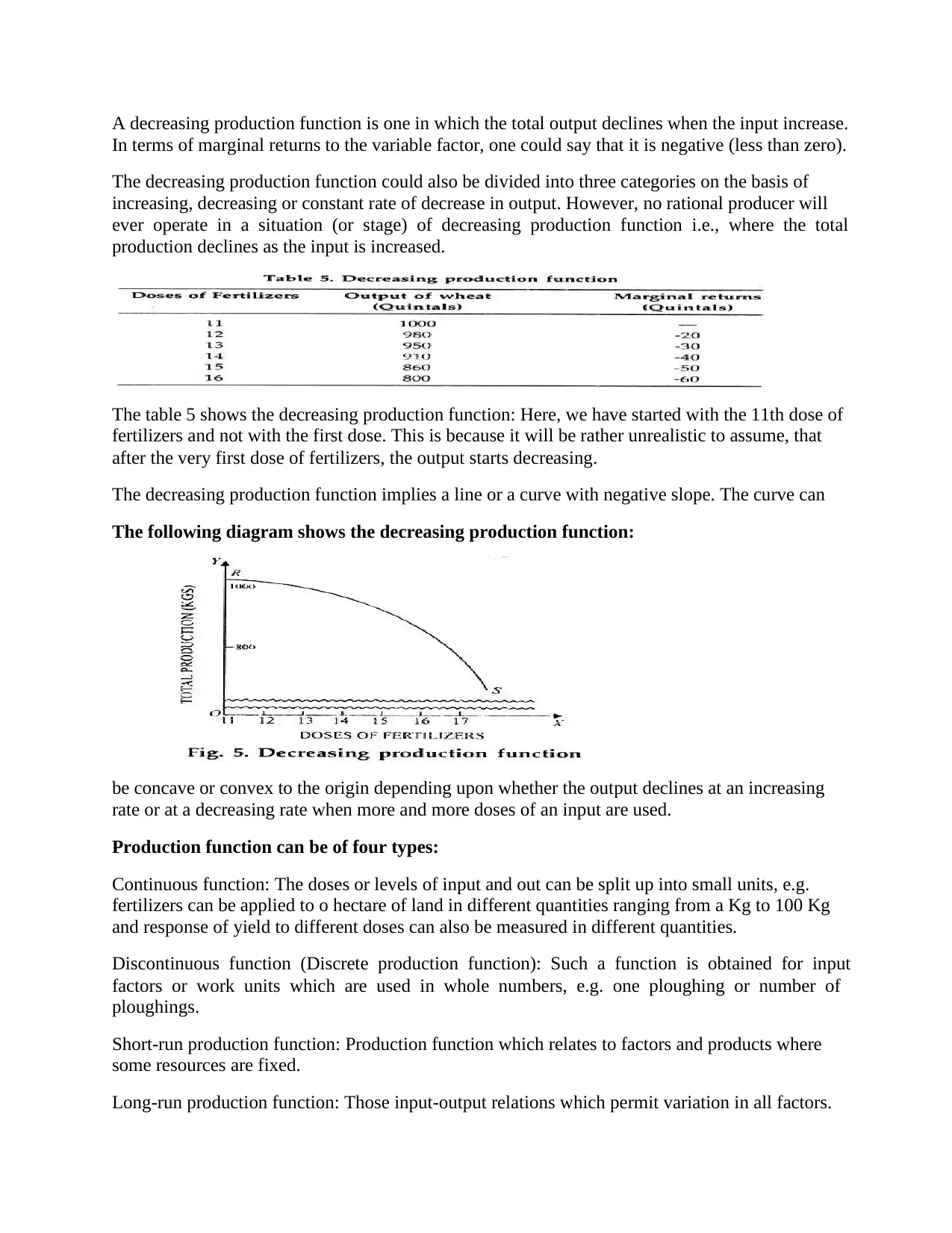
The table 5 shows the decreasing production function: Here, we have started with the 11th dose of
fertilizers and not with the first dose. This is because it will be rather unrealistic to assume, that
after the very first dose of fertilizers, the output starts decreasing.
The decreasing production function implies a line or a curve with negative slope. The curve can
The following diagram shows the decreasing production function:
be concave or convex to the origin depending upon whether the output declines at an increasing
rate or at a decreasing rate when more and more doses of an input are used.
Production function can be of four types:
Continuous function: The doses or levels of input and out can be split up into small units, e.g.
fertilizers can be applied to o hectare of land in different quantities ranging from a Kg to 100 Kg
and response of yield to different doses can also be measured in different quantities.
Discontinuous function (Discrete production function): Such a function is obtained for input
factors or work units which are used in whole numbers, e.g. one ploughing or number of
ploughings.
Short-run production function: Production function which relates to factors and products where
some resources are fixed.
Long-run production function: Those input-output relations which permit variation in all factors.

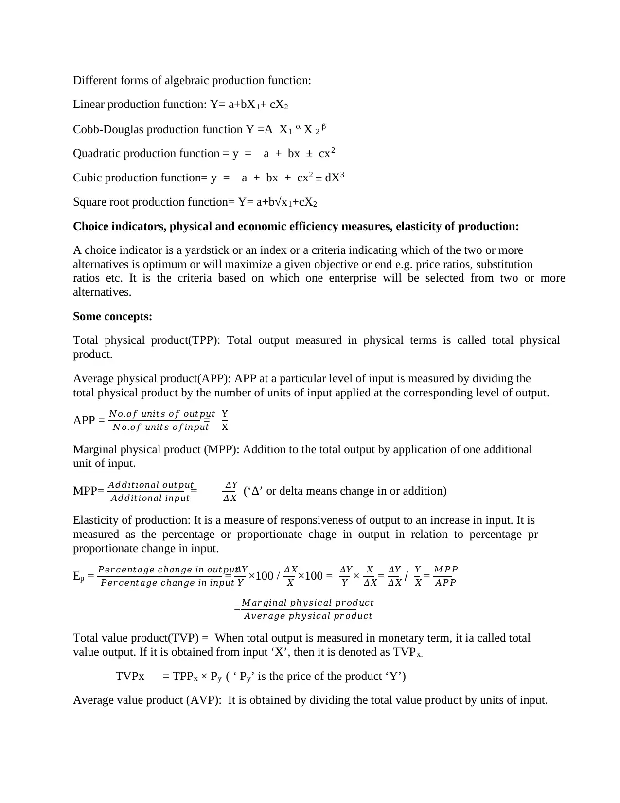
Different forms of algebraic production function:
Linear production function: Y= a+bX1+ cX2
Cobb-Douglas production function Y =A X1  X 2 
Quadratic production function = y = a + bx ± cx2
Cubic production function= y = a + bx + cx2 ± dX3
Square root production function= Y= a+b√x1+cX2
Choice indicators, physical and economic efficiency measures, elasticity of production:
A choice indicator is a yardstick or an index or a criteria indicating which of the two or more
alternatives is optimum or will maximize a given objective or end e.g. price ratios, substitution
ratios etc. It is the criteria based on which one enterprise will be selected from two or more
alternatives.
Some concepts:
Total physical product(TPP): Total output measured in physical terms is called total physical
product.
Average physical product(APP): APP at a particular level of input is measured by dividing the
total physical product by the number of units of input applied at the corresponding level of output.
APP = 𝑁𝑜.𝑜𝑓 𝑢𝑛𝑖𝑡𝑠 𝑜𝑓 𝑜𝑢𝑡𝑝𝑢𝑡
𝑁𝑜.𝑜𝑓 𝑢𝑛𝑖𝑡𝑠 𝑜𝑓𝑖𝑛𝑝𝑢𝑡
= Y
X
Marginal physical product (MPP): Addition to the total output by application of one additional
unit of input.
MPP= 𝐴𝑑𝑑𝑖𝑡𝑖𝑜𝑛𝑎𝑙 𝑜𝑢𝑡𝑝𝑢𝑡
𝐴𝑑𝑑𝑖𝑡𝑖𝑜𝑛𝑎𝑙 𝑖𝑛𝑝𝑢𝑡= 𝛥𝑌
𝛥𝑋 (‘Δ’ or delta means change in or addition)
Elasticity of production: It is a measure of responsiveness of output to an increase in input. It is
measured as the percentage or proportionate chage in output in relation to percentage pr
proportionate change in input.
Ep = 𝑃𝑒𝑟𝑐𝑒𝑛𝑡𝑎𝑔𝑒 𝑐ℎ𝑎𝑛𝑔𝑒 𝑖𝑛 𝑜𝑢𝑡𝑝𝑢𝑡
𝑃𝑒𝑟𝑐𝑒𝑛𝑡𝑎𝑔𝑒 𝑐ℎ𝑎𝑛𝑔𝑒 𝑖𝑛 𝑖𝑛𝑝𝑢𝑡
= 𝛥𝑌
𝑌 ×100 / 𝛥𝑋
𝑋 ×100 = 𝛥𝑌
𝑌 × 𝑋
𝛥𝑋= 𝛥𝑌
𝛥𝑋 / 𝑌
𝑋 = 𝑀𝑃𝑃
𝐴𝑃𝑃
=𝑀𝑎𝑟𝑔𝑖𝑛𝑎𝑙 𝑝ℎ𝑦𝑠𝑖𝑐𝑎𝑙 𝑝𝑟𝑜𝑑𝑢𝑐𝑡
𝐴𝑣𝑒𝑟𝑎𝑔𝑒 𝑝ℎ𝑦𝑠𝑖𝑐𝑎𝑙 𝑝𝑟𝑜𝑑𝑢𝑐𝑡
Total value product(TVP) = When total output is measured in monetary term, it ia called total
value output. If it is obtained from input ‘X’, then it is denoted as TVPx.
TVPx = TPPx × Py ( ‘ Py’ is the price of the product ‘Y’)
Average value product (AVP): It is obtained by dividing the total value product by units of input.

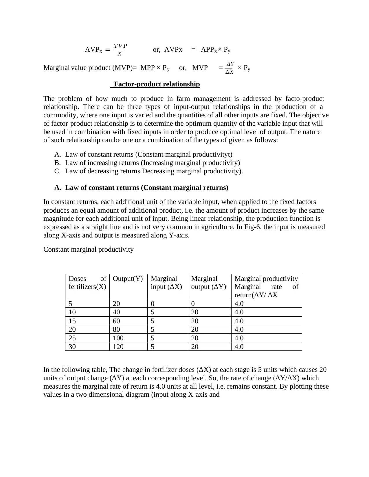
AVPx = 𝑇𝑉𝑃
𝑋 or, AVPx = APPx × Py
Marginal value product (MVP)= MPP × Py or, MVP = 𝛥𝑌
𝛥𝑋 × Py
Factor-product relationship
The problem of how much to produce in farm management is addressed by facto-product
relationship. There can be three types of input-output relationships in the production of a
commodity, where one input is varied and the quantities of all other inputs are fixed. The objective
of factor-product relationship is to determine the optimum quantity of the variable input that will
be used in combination with fixed inputs in order to produce optimal level of output. The nature
of such relationship can be one or a combination of the types of given as follows:
A. Law of constant returns (Constant marginal productivityt)
B. Law of increasing returns (Increasing marginal productivity)
C. Law of decreasing returns Decreasing marginal productivity).
A. Law of constant returns (Constant marginal returns)
In constant returns, each additional unit of the variable input, when applied to the fixed factors
produces an equal amount of additional product, i.e. the amount of product increases by the same
magnitude for each additional unit of input. Being linear relationship, the production function is
expressed as a straight line and is not very common in agriculture. In Fig-6, the input is measured
along X-axis and output is measured along Y-axis.
Constant marginal productivity
Doses of
fertilizers(X)
Output(Y) Marginal
input (ΔX)
Marginal
output (ΔY)
Marginal productivity
Marginal rate of
return(ΔY/ ΔX
5 20 0 0 4.0
10 40 5 20 4.0
15 60 5 20 4.0
20 80 5 20 4.0
25 100 5 20 4.0
30 120 5 20 4.0
In the following table, The change in fertilizer doses (ΔX) at each stage is 5 units which causes 20
units of output change (ΔY) at each corresponding level. So, the rate of change (ΔY/ΔX) which
measures the marginal rate of return is 4.0 units at all level, i.e. remains constant. By plotting these
values in a two dimensional diagram (input along X-axis and

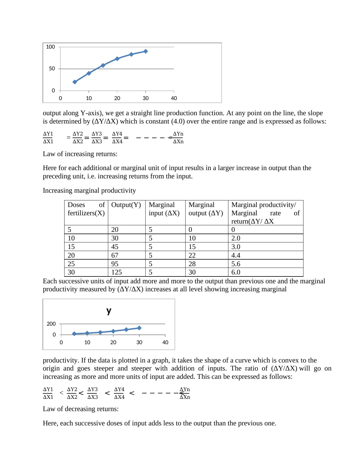
output along Y-axis), we get a straight line production function. At any point on the line, the slope
is determined by (ΔY/ΔX) which is constant (4.0) over the entire range and is expressed as follows:
ΔY1
ΔX1 = ΔY2
ΔX2 = ΔY3
ΔX3 = ΔY4
ΔX4 = − − − − −=ΔYn
ΔXn
Law of increasing returns:
Here for each additional or marginal unit of input results in a larger increase in output than the
preceding unit, i.e. increasing returns from the input.
Increasing marginal productivity
Doses of
fertilizers(X)
Output(Y) Marginal
input (ΔX)
Marginal
output (ΔY)
Marginal productivity/
Marginal rate of
return(ΔY/ ΔX
5 20 5 0 0
10 30 5 10 2.0
15 45 5 15 3.0
20 67 5 22 4.4
25 95 5 28 5.6
30 125 5 30 6.0
Each successive units of input add more and more to the output than previous one and the marginal
productivity measured by (ΔY/ΔX) increases at all level showing increasing marginal
productivity. If the data is plotted in a graph, it takes the shape of a curve which is convex to the
origin and goes steeper and steeper with addition of inputs. The ratio of (ΔY/ΔX) will go on
increasing as more and more units of input are added. This can be expressed as follows:
ΔY1
ΔX1 < ΔY2
ΔX2 < ΔY3
ΔX3 < ΔY4
ΔX4 < − − − − −<
ΔYn
ΔXn
Law of decreasing returns:
Here, each successive doses of input adds less to the output than the previous one.
0
50
100
0 10 20 30 40
0
200
0 10 20 30 40
y

Doses of
fertilizers(X)
Output(Y) Marginal
input (ΔX)
Marginal
output (ΔY)
Marginal productivity
Marginal rate of
return(ΔY/ ΔX
5 20 0 0 0
10 40 5 20 4.0
15 58 5 18 3.87
20 73 5 15 3.65
25 83 5 10 3.32
30 90 5 7 3.0
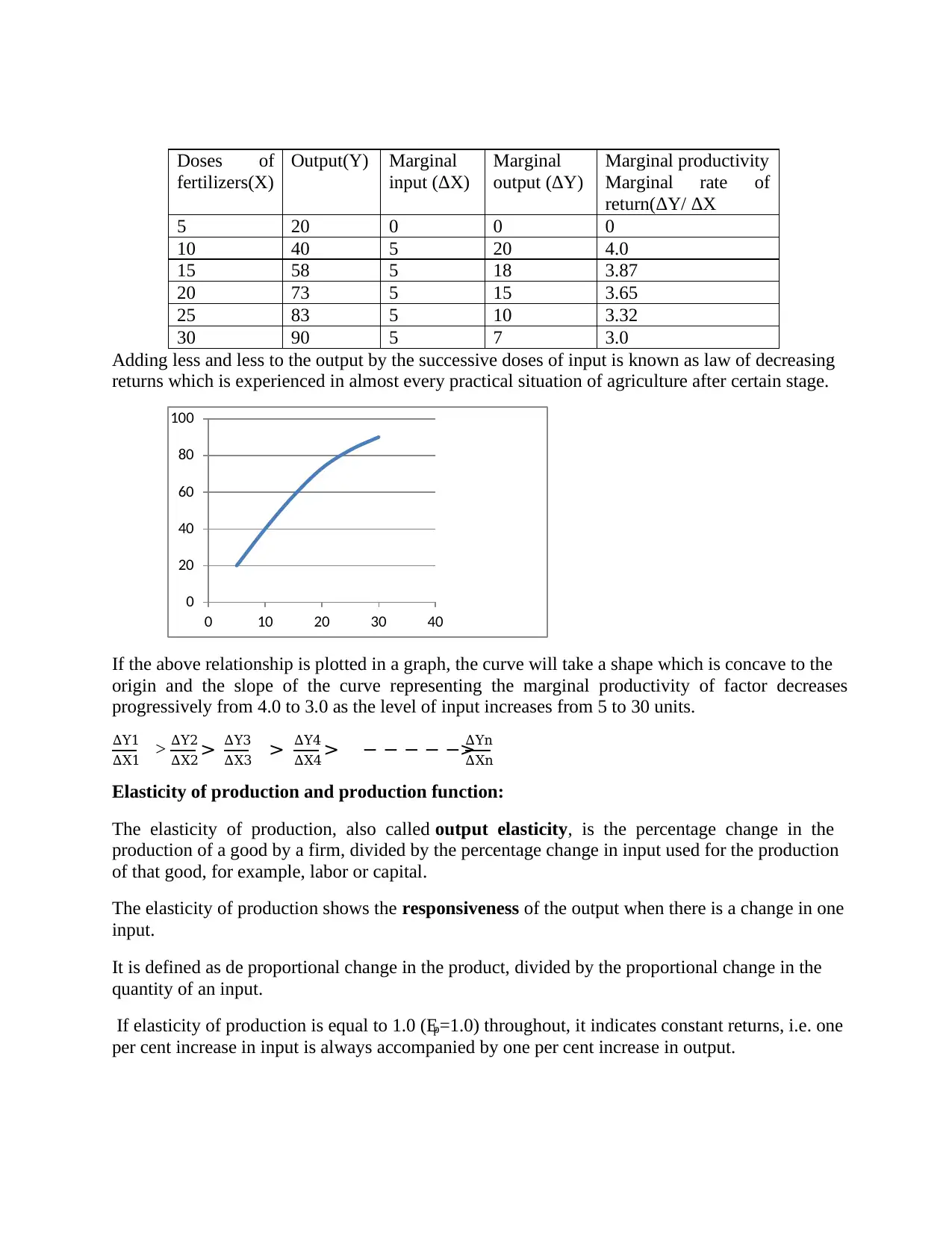
Adding less and less to the output by the successive doses of input is known as law of decreasing
returns which is experienced in almost every practical situation of agriculture after certain stage.
If the above relationship is plotted in a graph, the curve will take a shape which is concave to the
origin and the slope of the curve representing the marginal productivity of factor decreases
progressively from 4.0 to 3.0 as the level of input increases from 5 to 30 units.
ΔY1
ΔX1 > ΔY2
ΔX2 > ΔY3
ΔX3 > ΔY4
ΔX4 > − − − − −>
ΔYn
ΔXn
Elasticity of production and production function:
The elasticity of production, also called output elasticity, is the percentage change in the
production of a good by a firm, divided by the percentage change in input used for the production
of that good, for example, labor or capital.
The elasticity of production shows the responsiveness of the output when there is a change in one
input.
It is defined as de proportional change in the product, divided by the proportional change in the
quantity of an input.
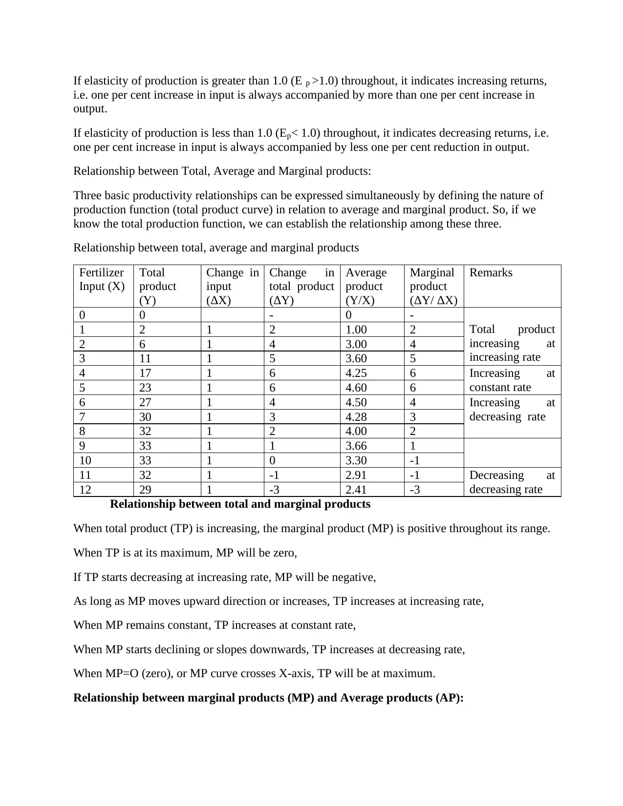
If elasticity of production is equal to 1.0 (Ep=1.0) throughout, it indicates constant returns, i.e. one
per cent increase in input is always accompanied by one per cent increase in output.
0
20
40
60
80
100
0 10 20 30 40

If elasticity of production is greater than 1.0 (E p >1.0) throughout, it indicates increasing returns,
i.e. one per cent increase in input is always accompanied by more than one per cent increase in
output.
If elasticity of production is less than 1.0 (Ep< 1.0) throughout, it indicates decreasing returns, i.e.
one per cent increase in input is always accompanied by less one per cent reduction in output.
Relationship between Total, Average and Marginal products:
Three basic productivity relationships can be expressed simultaneously by defining the nature of
production function (total product curve) in relation to average and marginal product. So, if we
know the total production function, we can establish the relationship among these three.
Relationship between total, average and marginal products
Fertilizer
Input (X)
Total
product
(Y)
Change in
input
(ΔX)
Change in
total product
(ΔY)
Average
product
(Y/X)
Marginal
product
(ΔY/ ΔX)
Remarks
0 0 - 0 -
Total product
increasing at
increasing rate
1 2 1 2 1.00 2
2 6 1 4 3.00 4
3 11 1 5 3.60 5
4 17 1 6 4.25 6 Increasing at
constant rate5 23 1 6 4.60 6
6 27 1 4 4.50 4 Increasing at
decreasing rate7 30 1 3 4.28 3
8 32 1 2 4.00 2
9 33 1 1 3.66 1
10 33 1 0 3.30 -1
11 32 1 -1 2.91 -1 Decreasing at
decreasing rate12 29 1 -3 2.41 -3
Relationship between total and marginal products
When total product (TP) is increasing, the marginal product (MP) is positive throughout its range.
When TP is at its maximum, MP will be zero,
If TP starts decreasing at increasing rate, MP will be negative,
As long as MP moves upward direction or increases, TP increases at increasing rate,
When MP remains constant, TP increases at constant rate,
When MP starts declining or slopes downwards, TP increases at decreasing rate,
When MP=O (zero), or MP curve crosses X-axis, TP will be at maximum.
Relationship between marginal products (MP) and Average products (AP):

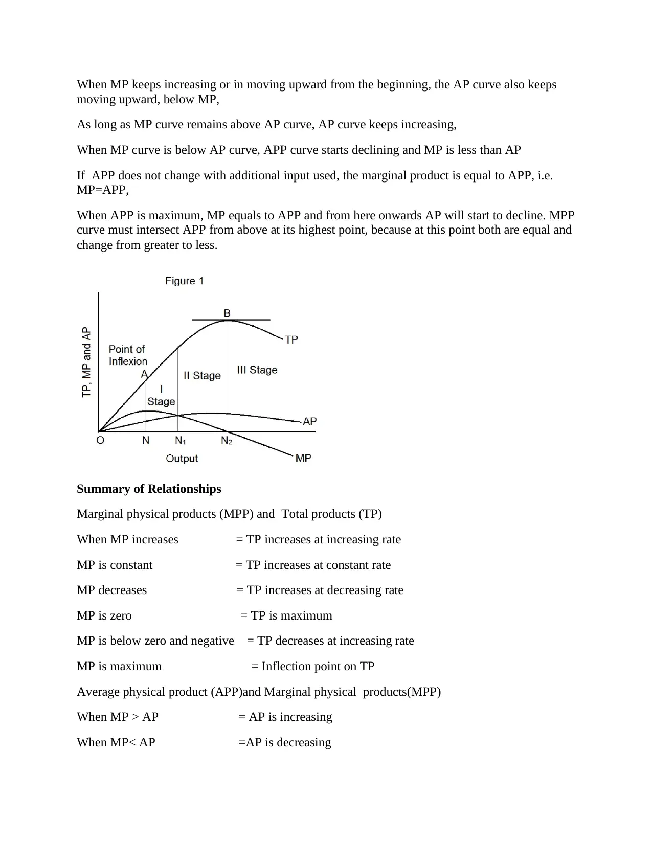
When MP keeps increasing or in moving upward from the beginning, the AP curve also keeps
moving upward, below MP,
As long as MP curve remains above AP curve, AP curve keeps increasing,
When MP curve is below AP curve, APP curve starts declining and MP is less than AP
If APP does not change with additional input used, the marginal product is equal to APP, i.e.
MP=APP,
When APP is maximum, MP equals to APP and from here onwards AP will start to decline. MPP
curve must intersect APP from above at its highest point, because at this point both are equal and
change from greater to less.
Summary of Relationships
Marginal physical products (MPP) and Total products (TP)
When MP increases = TP increases at increasing rate
MP is constant = TP increases at constant rate
MP decreases = TP increases at decreasing rate
MP is zero = TP is maximum
MP is below zero and negative = TP decreases at increasing rate
MP is maximum = Inflection point on TP
Average physical product (APP)and Marginal physical products(MPP)
When MP > AP = AP is increasing
When MP< AP =AP is decreasing

MP equals AP =AP is maximum
Law of variable proportion
The law of variable proportions states that as the quantity of one factor is increased, keeping the
other factors fixed, the marginal product of that factor will eventually decline. This means that
upto the use of a certain amount of variable factor, marginal product of the factor may increase
and after a certain stage it starts diminishing. When the variable factor becomes relatively
abundant, the marginal product may become negative.
Definition
“If the quantity of one productive service is increased by equal increments, with the quantity of
other resource services held constant, the increments to total product may increase at first but will
decrease after a certain point” – E.O.Heady
“An increase in capital and labour applied in cultivation of land causes in general, less than
proportionate increase in the amount of product raised, unless it happens to coincide with an
improvement in the arts of agriculture” - Marshall.
As the amount of variable resource used in production of a product is increased, the output of the
product will at first increase at an increasing rate, then increase at a decreasing rate and finally a
point will be reached, where further application of the variable resource will result in a decline in
the total output of production.
In short, marginal product of variable input will first increase, then decrease and finally become
negative.
Assumptions: The law of variable proportions holds good under the following conditions:
Constant Technology:
The state of technology is assumed to be given and constant. If there is an improvement in
technology the production function will move upward.
Factor Proportions are Variable:
The law assumes that factor proportions are variable. If factors of production are to be combined
in a fixed proportion, the law has no validity.
Homogeneous Factor Units:
The units of variable factor are homogeneous. Each unit is identical in quality and amount with
every other unit.
Short-Run: Short run refers to a period of time in which the supply of certain inputs (e.g. plant,
building and machines, etc.) is fixed or inelastic. In short run, therefore, production of a commodity
can be increased by increasing the use of variable inputs, like labour and raw materials. The law
operates in the short-run when it is not possible to vary all factor inputs.

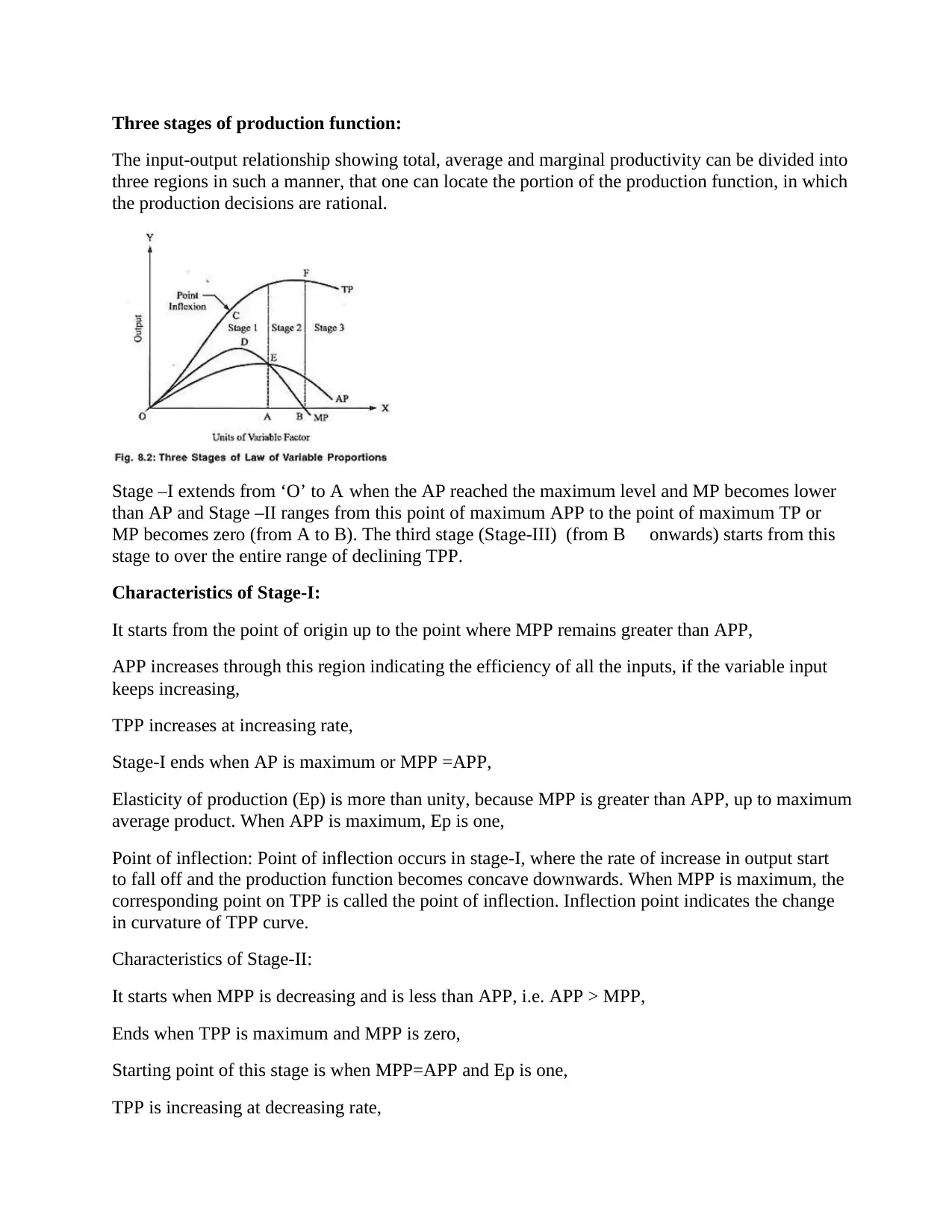
Three stages of production function:
The input-output relationship showing total, average and marginal productivity can be divided into
three regions in such a manner, that one can locate the portion of the production function, in which
the production decisions are rational.
Stage –I extends from ‘O’ to A when the AP reached the maximum level and MP becomes lower
than AP and Stage –II ranges from this point of maximum APP to the point of maximum TP or
MP becomes zero (from A to B). The third stage (Stage-III) (from B onwards) starts from this
stage to over the entire range of declining TPP.
Characteristics of Stage-I:
It starts from the point of origin up to the point where MPP remains greater than APP,
APP increases through this region indicating the efficiency of all the inputs, if the variable input
keeps increasing,
TPP increases at increasing rate,
Stage-I ends when AP is maximum or MPP =APP,
Elasticity of production (Ep) is more than unity, because MPP is greater than APP, up to maximum
average product. When APP is maximum, Ep is one,
Point of inflection: Point of inflection occurs in stage-I, where the rate of increase in output start
to fall off and the production function becomes concave downwards. When MPP is maximum, the
corresponding point on TPP is called the point of inflection. Inflection point indicates the change
in curvature of TPP curve.
Characteristics of Stage-II:
It starts when MPP is decreasing and is less than APP, i.e. APP > MPP,
Ends when TPP is maximum and MPP is zero,
Starting point of this stage is when MPP=APP and Ep is one,
TPP is increasing at decreasing rate,

Optimum point of input use is in this rational region.
If the producer wants to maximize their output, he must operate in region-2 (Stage-II) of production
function,
Elasticity of production is less than one, but greater than zero between maximum APP and
maximum TPP.
Characteristics of Stage-III:
TPP decreases, but it is still positive
MPP crosses zero point and becomes negative,
It is not profitable zone, additional quantity of input reduces TPP,
Ep is less than zero as TPP declines,
Double loss---Irrational zone
Reduced production
Unnecessary additional cost of production
Irrational and rational stages of production function
Irrational production exists if there is any possibility for the rearrangement of resources, either to
get a greater product from the same level of input or to get the same product with smaller amount
of resources. In stage-I, the average productivity of variable resources keep increasing and profit
can always be increased. Instead of reducing the application of variable resources to fixed factors
in stage-I, the farmers can always obtain more product and profits from the same resources. In
stage –III, the average product decreases further, marginal product becomes negative and total
product is decreasing, showing inefficient use of resources.
Therefore, the farmer should stay between the points of maximum average product and zero
marginal product (maximum total product), where Ep is less than one but greater than zero which
indicates the stage-II. The optimum level of resource use must fall in this region of economic
relevance. The optimum point of resource use or the profit maximizing amount of product can be
decided only with the help of choice indicator, i.e. factor-product prices.
Alternative line of thought
A rational producer will not like to operate in stage-I, because in this stage AP is continuously
rising, if he stops it means he is not taking full advantage of consistently rising productivity.
The firm can earn more profit by hiring more variable output and increasing his AP.
So more can be earn if a rational producer wants to earn more, and hence he will not like to operate
in this stage. A rational producer will not like to operate in stage III too, because in this stage MP
is negative, thus producer can increase his TP by employing less of the variable factor, as more of
variable factors result in decrease in output. So a rational producer will not incur expenditure in

employing additional factor if it result in decrease in output. Farmers will not like to operate in
this stage. By the process of elimination, we come to the conclusion that a rational producer will
operate in stage II, as here TP is maximum and MP is Zero.
Limitations of the law:
Improved methods of cultivation: New techniques of crop production can bring about increasing
returns. But when these techniques reach saturation without further improvements, the law must
operate.
New soils: When a virgin soil is brought under cultivation, the additional return from successive
dose of labour and capital may increase for time in the beginning.
Insufficient capital: Under limited capital conditions, sometimes the farmers operate in stage-I, a
gradual increase in capital application yields more than proportionate return. Later, the decreasing
return sets in.
Profit maximizing criteria:
Two methods are available for defining maximum profits;
Profit from the use of factor is maximized when the marginal product is equated to the price ratio,
and
Profits are maximized for the fixed unit if the marginal value productivity of factor is equal to
marginal cost of the factor.
Suppose, a farmer produces an output, ‘Y’ by using an input, ‘X’ and the farm is operating under
perfect condition. The product and factor market is assumed to be purely competitive and the prices
of output and input are represented by Py and Px. The total revenue (TR) obtained from the sale of
the output ‘Y’ is the same as Y×Py which is sometimes referred to as the total value of the product
(TVP). Similarly by multiplying the amount of input ‘X’ by price P x, we get the total factor cost
(TFC) which is equal to X * P x. Profit (Π) is the total value of the product (TVP) less the total
factor cost (TFC). The profit function for the farmer can be written as: