Rejecting the Null Hypothesis: House Dwelling Type

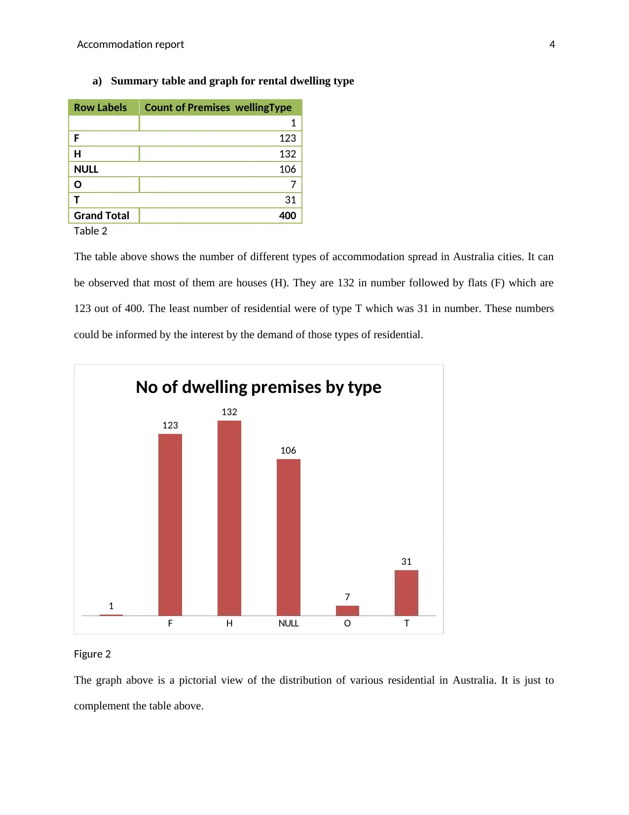
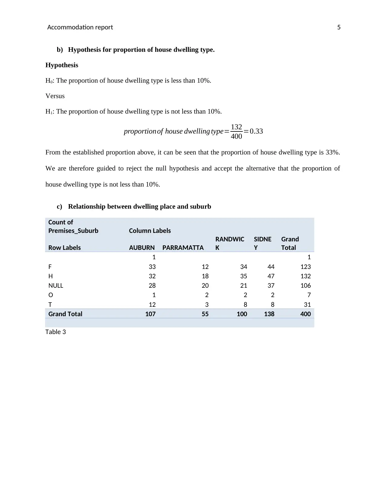
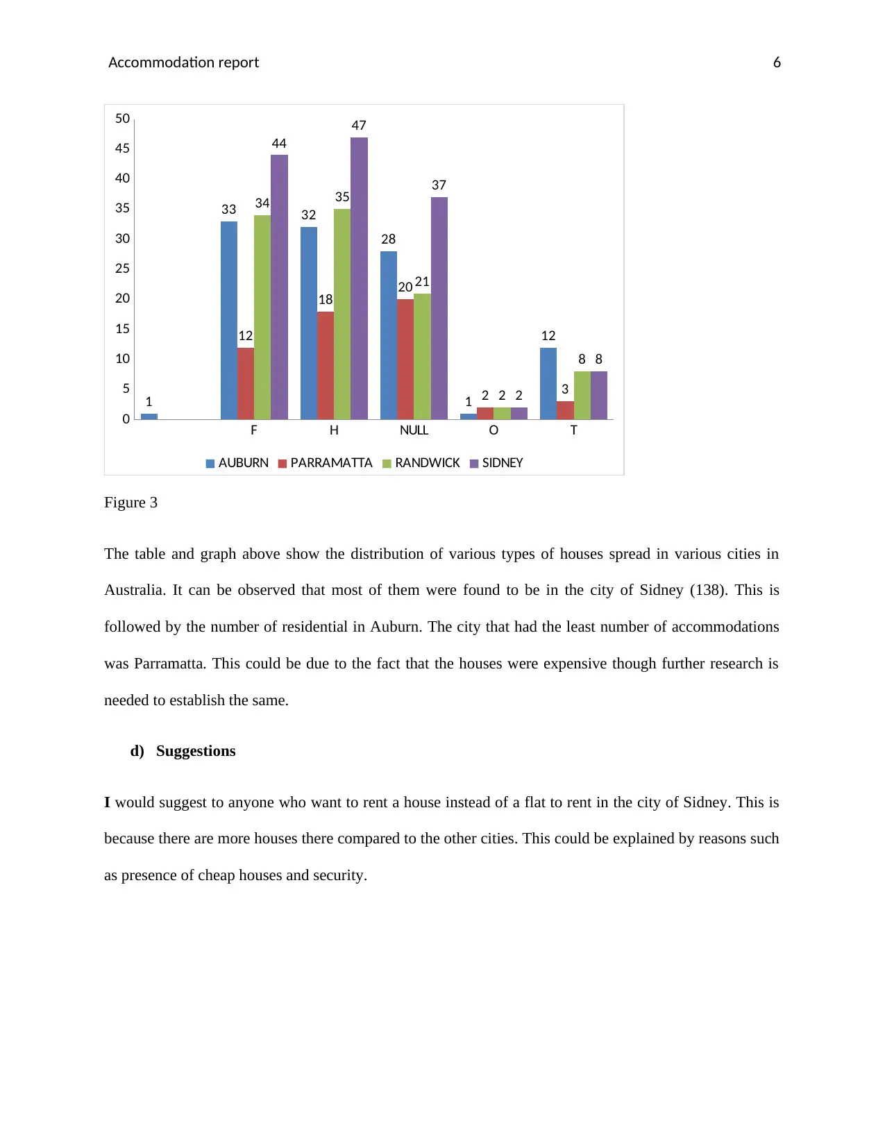
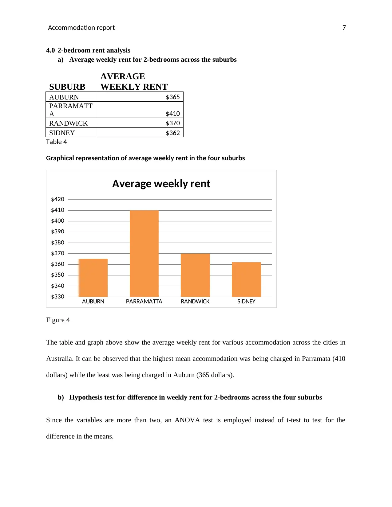
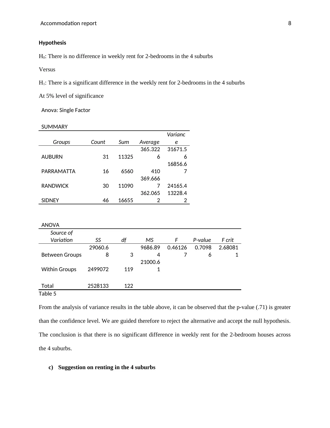
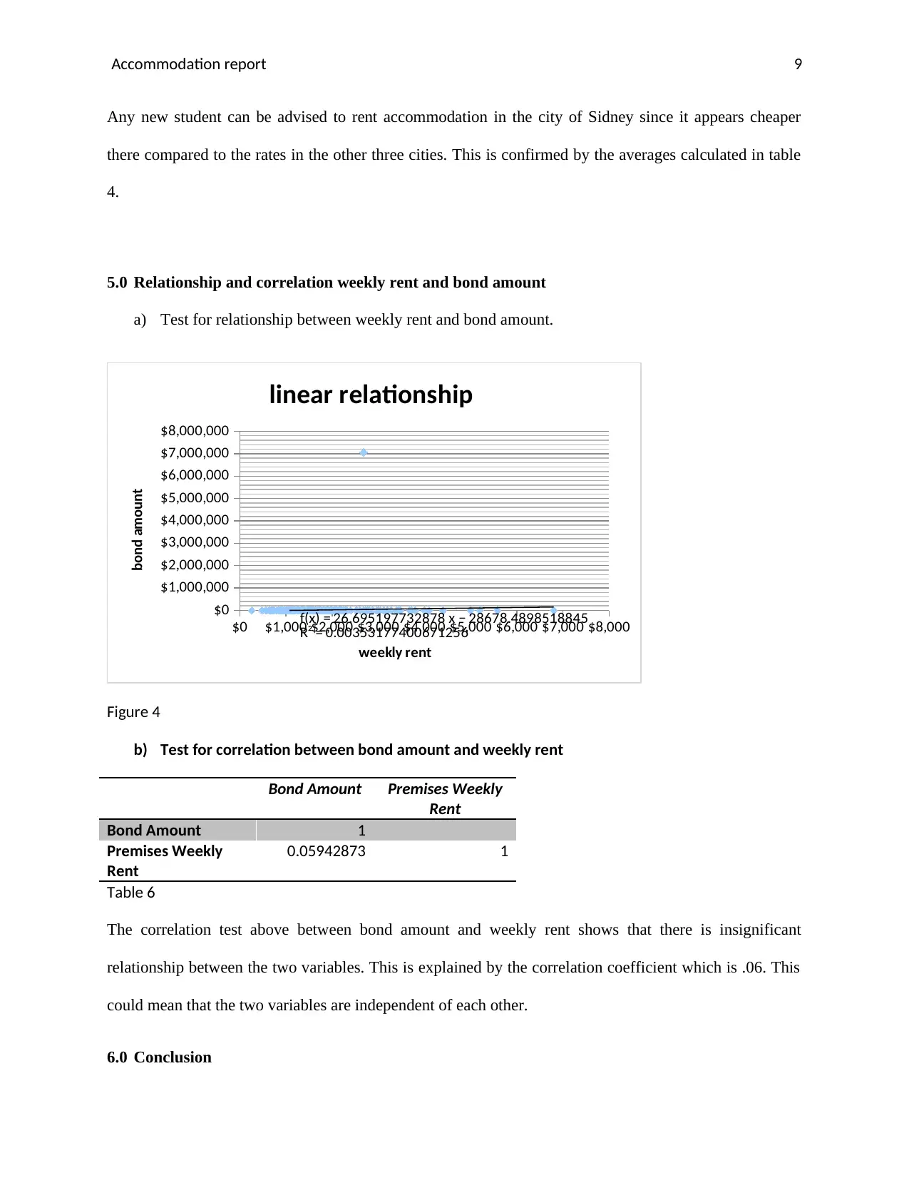
The table and graph show the distribution of houses in different cities in Australia, with Sidney having the most (138) followed by Auburn. The analysis also shows the average weekly rent for 2-bedroom houses across suburbs, with Parramatta having the highest rate ($410). An ANOVA test found no significant difference in weekly rent rates across the four suburbs. Finally, a correlation test revealed no significant relationship between bond amount and weekly rent.

Accommodation report 1
Name:
Institution:
Date:
Accommodation report on Australian cities

Accommodation report 2
1.0 INTRODUCTION
This survey report is focused on giving information after an analysis about rent in different parts of
Australia. This information is helpful to international travellers and more so international students who
seek education in various cities in Australia. It forms a basis of decision making when it comes to
choosing the type of accommodation that is suitable for any particular individual. This research depended
entirely on secondary data as it did not collect its own information. The data was sourced from
department of finance services and innovation of Australia. The data had both numerical variables and
nominal variables. Some of the numerical variables were bond amount in dollars and weekly rent in
dollars. The sample obtained for this report was not biased but large enough to representative the entire
population. The sample size was 400.
2.0 INTERNATIONAL STUDENTS WEEKLY RENT
a) Descriptive summary of students’ weekly rent
descriptive statistics for weekly rent
Mean 18197.98992
Standard Error 17785.78627
Median 395
Mode 0
Standard Deviation 354379.2809
Sample Variance 1.25585E+11
Kurtosis 396.9994654
Skewness 19.92483878
Range 7061367
Minimum 0
Maximum 7061367
Sum 7224602
Count 397
Table 1
As can be observed from the table above, the mean weekly rent in dollars is 18197.99. The maximum rent
charged weekly in dollars is 7,061,367
b) Distribution

Accommodation report 3
The data set is skewed to the right so much. This is because it has a skewness value of 19.92. It can also
be seen that the distribution is highly kurtic. This means that it has a very sharp apex on its curve. This
could be due to having very extreme high values like outliers which then affect the measures of central
tendencies of the data such as mean, mode and median. To check for the presence of outliers, a scatter
plot of the data was generated and is as below;
$0 $1,000 $2,000 $3,000 $4,000 $5,000 $6,000 $7,000 $8,000
$0
$1,000,000
$2,000,000
$3,000,000
$4,000,000
$5,000,000
$6,000,000
$7,000,000
$8,000,000
f(x) = 26.695197732878 x − 28678.4898518845
R² = 0.00353177400671256
scatterplot for weekly rent
weekly rent
bond amount
Figure 1
As can be observed from figure 1 above, there is an extremely large value in the data set. This value is
7,061,367 dollars. This value makes the measures of central tendencies such as the mean not to depict the
real picture of the data since they are adversely affected by this extreme value. Therefore the mean rent
could be much lower than what is given in the descriptive table. To get the real mean rent that can be used
as a basis of making decision for students who want accommodation, then this extreme value is omitted.
3.0 Rental – dwelling type

Accommodation report 4
a) Summary table and graph for rental dwelling type
Row Labels Count of Premises wellingType
1
F 123
H 132
NULL 106
O 7
T 31
Grand Total 400
Table 2
The table above shows the number of different types of accommodation spread in Australia cities. It can
be observed that most of them are houses (H). They are 132 in number followed by flats (F) which are
123 out of 400. The least number of residential were of type T which was 31 in number. These numbers
could be informed by the interest by the demand of those types of residential.
F H NULL O T
1
123
132
106
7
31
No of dwelling premises by type
Figure 2
The graph above is a pictorial view of the distribution of various residential in Australia. It is just to
complement the table above.

Accommodation report 5
b) Hypothesis for proportion of house dwelling type.
Hypothesis
H0: The proportion of house dwelling type is less than 10%.
Versus
H1: The proportion of house dwelling type is not less than 10%.
proportionof house dwelling type= 132
400 =0.33
From the established proportion above, it can be seen that the proportion of house dwelling type is 33%.
We are therefore guided to reject the null hypothesis and accept the alternative that the proportion of
house dwelling type is not less than 10%.
c) Relationship between dwelling place and suburb
Count of
Premises_Suburb Column Labels
Row Labels AUBURN PARRAMATTA
RANDWIC
K
SIDNE
Y
Grand
Total
1 1
F 33 12 34 44 123
H 32 18 35 47 132
NULL 28 20 21 37 106
O 1 2 2 2 7
T 12 3 8 8 31
Grand Total 107 55 100 138 400
Table 3

Accommodation report 6
F H NULL O T
0
5
10
15
20
25
30
35
40
45
50
1
33 32
28
1
1212
18 20
2 3
34 35
21
2
8
44
47
37
2
8
AUBURN PARRAMATTA RANDWICK SIDNEY
Figure 3
The table and graph above show the distribution of various types of houses spread in various cities in
Australia. It can be observed that most of them were found to be in the city of Sidney (138). This is
followed by the number of residential in Auburn. The city that had the least number of accommodations
was Parramatta. This could be due to the fact that the houses were expensive though further research is
needed to establish the same.
d) Suggestions
I would suggest to anyone who want to rent a house instead of a flat to rent in the city of Sidney. This is
because there are more houses there compared to the other cities. This could be explained by reasons such
as presence of cheap houses and security.

Accommodation report 7
4.0 2-bedroom rent analysis
a) Average weekly rent for 2-bedrooms across the suburbs
SUBURB
AVERAGE
WEEKLY RENT
AUBURN $365
PARRAMATT
A $410
RANDWICK $370
SIDNEY $362
Table 4
Graphical representation of average weekly rent in the four suburbs
AUBURN PARRAMATTA RANDWICK SIDNEY
$330
$340
$350
$360
$370
$380
$390
$400
$410
$420
Average weekly rent
Figure 4
The table and graph above show the average weekly rent for various accommodation across the cities in
Australia. It can be observed that the highest mean accommodation was being charged in Parramata (410
dollars) while the least was being charged in Auburn (365 dollars).
b) Hypothesis test for difference in weekly rent for 2-bedrooms across the four suburbs
Since the variables are more than two, an ANOVA test is employed instead of t-test to test for the
difference in the means.

Accommodation report 8
Hypothesis
H0: There is no difference in weekly rent for 2-bedrooms in the 4 suburbs
Versus
H1: There is a significant difference in the weekly rent for 2-bedrooms in the 4 suburbs
At 5% level of significance
Anova: Single Factor
SUMMARY
Groups Count Sum Average
Varianc
e
AUBURN 31 11325
365.322
6
31671.5
6
PARRAMATTA 16 6560 410
16856.6
7
RANDWICK 30 11090
369.666
7 24165.4
SIDNEY 46 16655
362.065
2
13228.4
2
ANOVA
Source of
Variation SS df MS F P-value F crit
Between Groups
29060.6
8 3
9686.89
4
0.46126
7
0.7098
6
2.68081
1
Within Groups 2499072 119
21000.6
1
Total 2528133 122
Table 5
From the analysis of variance results in the table above, it can be observed that the p-value (.71) is greater
than the confidence level. We are guided therefore to reject the alternative and accept the null hypothesis.
The conclusion is that there is no significant difference in weekly rent for the 2-bedroom houses across
the 4 suburbs.
c) Suggestion on renting in the 4 suburbs

Accommodation report 9
Any new student can be advised to rent accommodation in the city of Sidney since it appears cheaper
there compared to the rates in the other three cities. This is confirmed by the averages calculated in table
4.
5.0 Relationship and correlation weekly rent and bond amount
a) Test for relationship between weekly rent and bond amount.
$0 $1,000 $2,000 $3,000 $4,000 $5,000 $6,000 $7,000 $8,000
$0
$1,000,000
$2,000,000
$3,000,000
$4,000,000
$5,000,000
$6,000,000
$7,000,000
$8,000,000
f(x) = 26.695197732878 x − 28678.4898518845
R² = 0.00353177400671256
linear relationship
weekly rent
bond amount
Figure 4
b) Test for correlation between bond amount and weekly rent
Bond Amount Premises Weekly
Rent
Bond Amount 1
Premises Weekly
Rent
0.05942873 1
Table 6
The correlation test above between bond amount and weekly rent shows that there is insignificant
relationship between the two variables. This is explained by the correlation coefficient which is .06. This
could mean that the two variables are independent of each other.
6.0 Conclusion

Accommodation report
10
From the analyses above, it can be concluded that weekly accommodation rates are almost the same in all
the four cities in Australia. This is so since there was no wide variance among them. An analysis of
variance performed on the rates of 2-bedrooms also suggested that there is no significant difference in the
rates of the same 2-bedrooms across the four cities in Australia. The research has also informed that bond
amounts and weekly rents do not affect each other and that they are independent.