Accounting and Finance

This project report covers topics such as calculation of monthly deposit, investment decision, assets calculations, real rate of interest, Australian housing market, risk definition, Australian credit system, calculation of BHP monthly return, and more.

Running Head: Accounting and Finance
1
Project Report: Accounting and Finance

Accounting and Finance
2
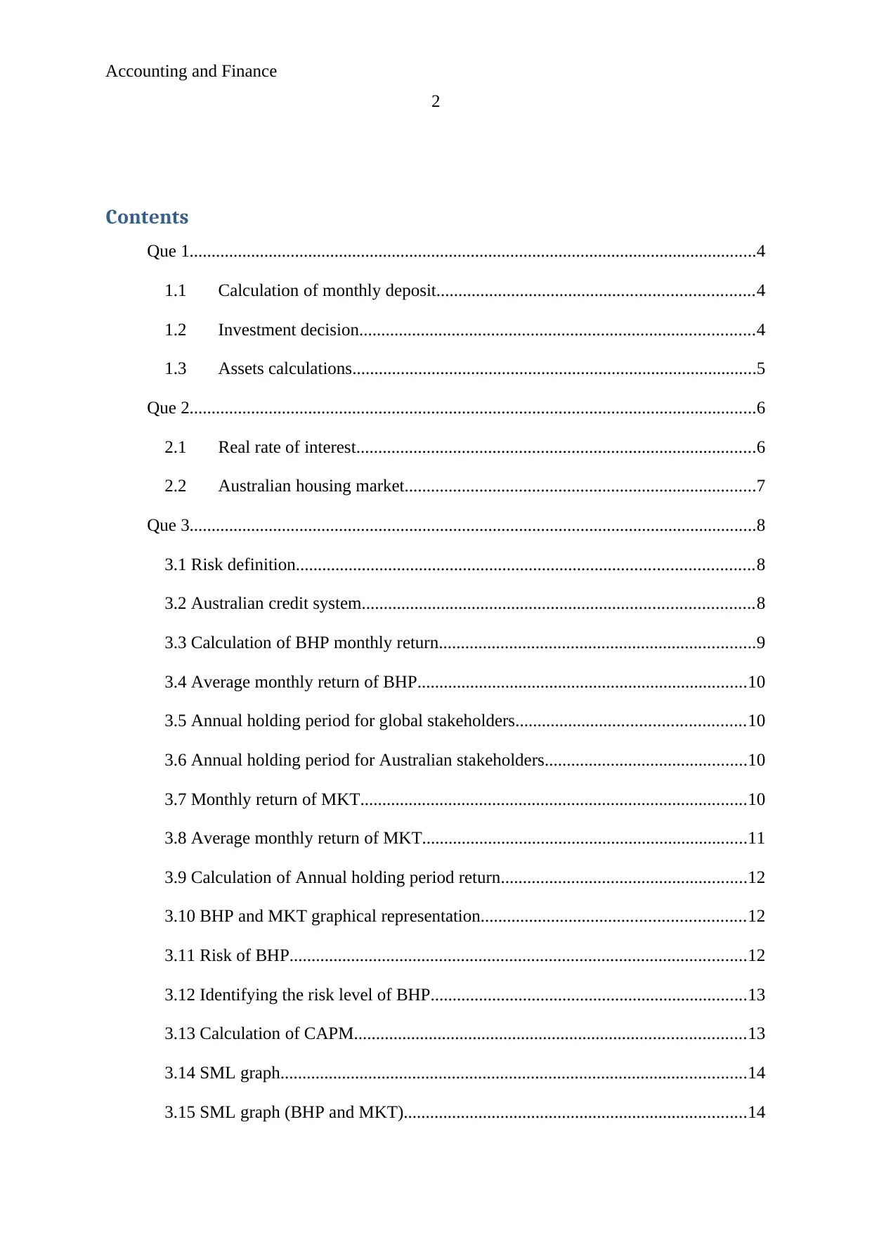
Contents
Que 1.................................................................................................................................4
1.1 Calculation of monthly deposit........................................................................4
1.2 Investment decision..........................................................................................4
1.3 Assets calculations............................................................................................5
Que 2.................................................................................................................................6
2.1 Real rate of interest...........................................................................................6
2.2 Australian housing market................................................................................7
Que 3.................................................................................................................................8
3.1 Risk definition........................................................................................................8
3.2 Australian credit system.........................................................................................8
3.3 Calculation of BHP monthly return........................................................................9
3.4 Average monthly return of BHP...........................................................................10
3.5 Annual holding period for global stakeholders....................................................10
3.6 Annual holding period for Australian stakeholders..............................................10
3.7 Monthly return of MKT........................................................................................10
3.8 Average monthly return of MKT..........................................................................11
3.9 Calculation of Annual holding period return........................................................12
3.10 BHP and MKT graphical representation............................................................12
3.11 Risk of BHP........................................................................................................12
3.12 Identifying the risk level of BHP........................................................................13
3.13 Calculation of CAPM.........................................................................................13
3.14 SML graph..........................................................................................................14
3.15 SML graph (BHP and MKT)..............................................................................14

Accounting and Finance
3
3.16 Portfolio’s return and beta..................................................................................15
References.......................................................................................................................16

Accounting and Finance
4
Que 1:
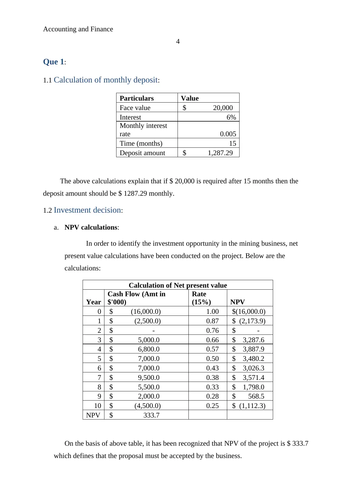
1.1 Calculation of monthly deposit:
Particulars Value
Face value $ 20,000
Interest 6%
Monthly interest
rate 0.005
Time (months) 15
Deposit amount $ 1,287.29
The above calculations explain that if $ 20,000 is required after 15 months then the
deposit amount should be $ 1287.29 monthly.
1.2 Investment decision:
a. NPV calculations:
In order to identify the investment opportunity in the mining business, net
present value calculations have been conducted on the project. Below are the
calculations:
Calculation of Net present value
Year
Cash Flow (Amt in
$'000)
Rate
(15%) NPV
0 $ (16,000.0) 1.00 $(16,000.0)
1 $ (2,500.0) 0.87 $ (2,173.9)
2 $ - 0.76 $ -
3 $ 5,000.0 0.66 $ 3,287.6
4 $ 6,800.0 0.57 $ 3,887.9
5 $ 7,000.0 0.50 $ 3,480.2
6 $ 7,000.0 0.43 $ 3,026.3
7 $ 9,500.0 0.38 $ 3,571.4
8 $ 5,500.0 0.33 $ 1,798.0
9 $ 2,000.0 0.28 $ 568.5
10 $ (4,500.0) 0.25 $ (1,112.3)
NPV $ 333.7
On the basis of above table, it has been recognized that NPV of the project is $ 333.7
which defines that the proposal must be accepted by the business.

Accounting and Finance
5
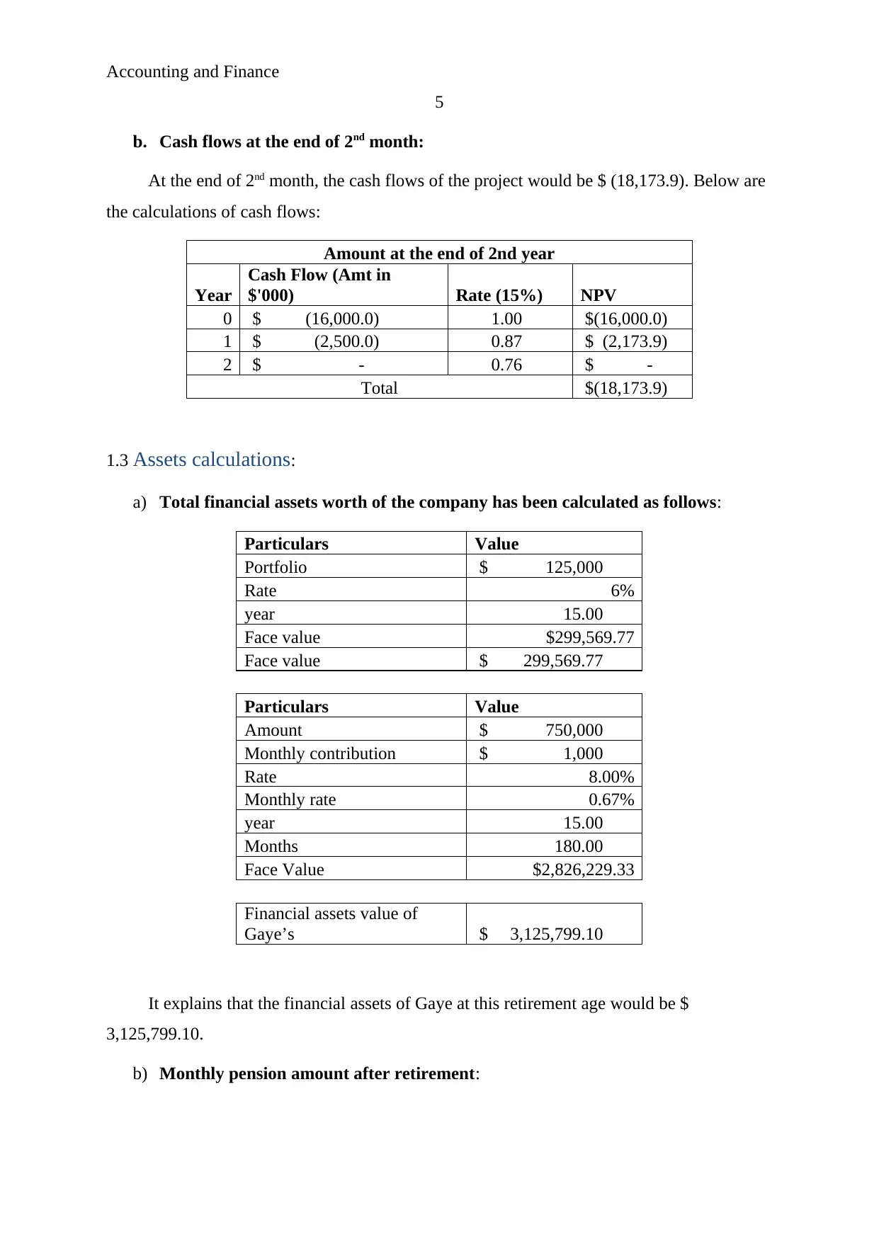
b. Cash flows at the end of 2nd month:
At the end of 2nd month, the cash flows of the project would be $ (18,173.9). Below are
the calculations of cash flows:
Amount at the end of 2nd year
Year
Cash Flow (Amt in
$'000) Rate (15%) NPV
0 $ (16,000.0) 1.00 $(16,000.0)
1 $ (2,500.0) 0.87 $ (2,173.9)
2 $ - 0.76 $ -
Total $(18,173.9)
1.3 Assets calculations:
a) Total financial assets worth of the company has been calculated as follows:
Particulars Value
Portfolio $ 125,000
Rate 6%
year 15.00
Face value $299,569.77
Face value $ 299,569.77
Particulars Value
Amount $ 750,000
Monthly contribution $ 1,000
Rate 8.00%
Monthly rate 0.67%
year 15.00
Months 180.00
Face Value $2,826,229.33
Financial assets value of
Gaye’s $ 3,125,799.10
It explains that the financial assets of Gaye at this retirement age would be $
3,125,799.10.
b) Monthly pension amount after retirement:

Accounting and Finance
6
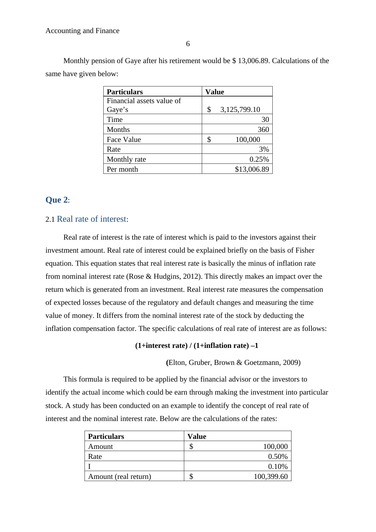
Monthly pension of Gaye after his retirement would be $ 13,006.89. Calculations of the
same have given below:
Particulars Value
Financial assets value of
Gaye’s $ 3,125,799.10
Time 30
Months 360
Face Value $ 100,000
Rate 3%
Monthly rate 0.25%
Per month $13,006.89
Que 2:
2.1 Real rate of interest:
Real rate of interest is the rate of interest which is paid to the investors against their
investment amount. Real rate of interest could be explained briefly on the basis of Fisher
equation. This equation states that real interest rate is basically the minus of inflation rate
from nominal interest rate (Rose & Hudgins, 2012). This directly makes an impact over the
return which is generated from an investment. Real interest rate measures the compensation
of expected losses because of the regulatory and default changes and measuring the time
value of money. It differs from the nominal interest rate of the stock by deducting the
inflation compensation factor. The specific calculations of real rate of interest are as follows:
(1+interest rate) / (1+inflation rate) –1
(Elton, Gruber, Brown & Goetzmann, 2009)
This formula is required to be applied by the financial advisor or the investors to
identify the actual income which could be earn through making the investment into particular
stock. A study has been conducted on an example to identify the concept of real rate of
interest and the nominal interest rate. Below are the calculations of the rates:
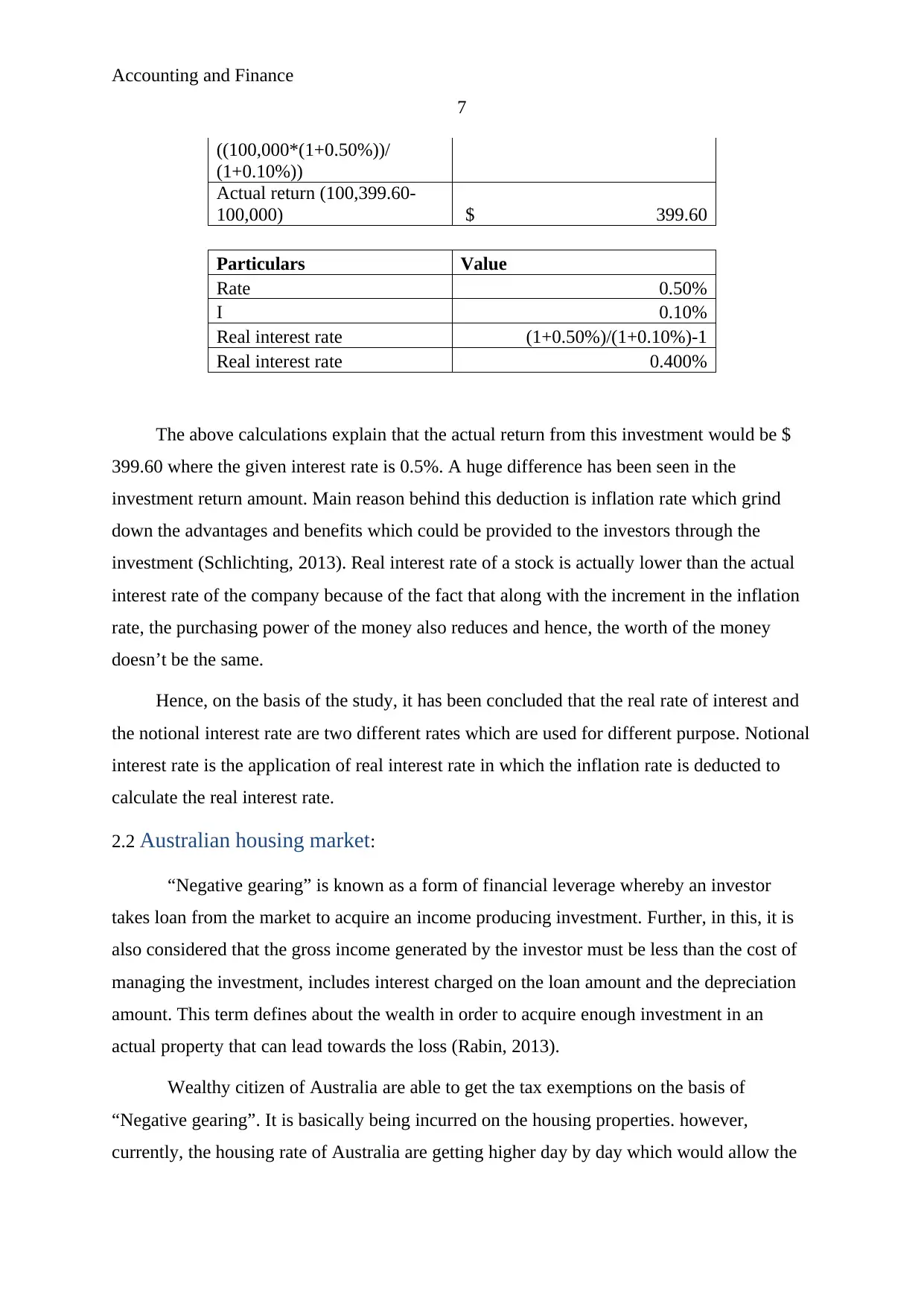
Particulars Value
Amount $ 100,000
Rate 0.50%
I 0.10%
Amount (real return) $ 100,399.60

Accounting and Finance
7
((100,000*(1+0.50%))/
(1+0.10%))
Actual return (100,399.60-
100,000) $ 399.60
Particulars Value
Rate 0.50%
I 0.10%
Real interest rate (1+0.50%)/(1+0.10%)-1
Real interest rate 0.400%
The above calculations explain that the actual return from this investment would be $
399.60 where the given interest rate is 0.5%. A huge difference has been seen in the
investment return amount. Main reason behind this deduction is inflation rate which grind
down the advantages and benefits which could be provided to the investors through the
investment (Schlichting, 2013). Real interest rate of a stock is actually lower than the actual
interest rate of the company because of the fact that along with the increment in the inflation
rate, the purchasing power of the money also reduces and hence, the worth of the money
doesn’t be the same.
Hence, on the basis of the study, it has been concluded that the real rate of interest and
the notional interest rate are two different rates which are used for different purpose. Notional
interest rate is the application of real interest rate in which the inflation rate is deducted to
calculate the real interest rate.
2.2 Australian housing market:
“Negative gearing” is known as a form of financial leverage whereby an investor
takes loan from the market to acquire an income producing investment. Further, in this, it is
also considered that the gross income generated by the investor must be less than the cost of
managing the investment, includes interest charged on the loan amount and the depreciation
amount. This term defines about the wealth in order to acquire enough investment in an
actual property that can lead towards the loss (Rabin, 2013).
Wealthy citizen of Australia are able to get the tax exemptions on the basis of
“Negative gearing”. It is basically being incurred on the housing properties. however,
currently, the housing rate of Australia are getting higher day by day which would allow the

Accounting and Finance
8
wealthy and rich people to get the better and higher return then previous return from the
investment.
Nevertheless, various arguments about the “negative gearing” in Australian housing
market has been studied and it has been found that various researches are against of “negative
gearing’ and some of them are supporting it. Some explains that tax deductions are got by the
people because they actually face loss because of the property whereas the other argues that
the “negative gearing” creates bubble in the market (Palicka, 2011).
To conclude, it has been measured that this is not ethical process for the Australian
market as it could lead the market towards the financial crisis similar to 2008. Due to the fact
that this allows the wealthy people to reduce their tax burden and improves their wealth.
Hence, it is recommended to the government and tax regulators to reduce the impact of
“negative gearing” from the market to set the stability and reduce the chances of financial
crisis (Madura, 2014).
Que 3:
3.1 Risk definition:
Investment risk could be defined as the chances of loss occurrences relative to the
total expected return from a particular investment. It is basically a measurement to identify
the uncertainty level of achieving the return as per the market and investors’ expectation. It is
the extent of unexpected outcomes which are to be realized by the investors. Risk attributes
could be seen differently by different investors such as conservative investors would see it as
a bad factor whereas a growth investor would find it as an opportunity to earn more return
from the investment (Higgins, 2012). In the investment perspective, risk could be considered
as the return parallel from an investment.
It is common saying that the higher the risk, higher the return from the investment
would be. CAPM calculations are conducted by the investors to measure the total return from
the investment on the basis of the risk level. Beta is basically used by the investors to identify
the risk level of an investment. Beta factor is used to describe the level of volatility in the
stock prices of an organization In comparison with the market index. Hence, it could be said
that if an investor wants to earn higher return from the market then the investors is required to
face higher risk in the market whereas if an investors don’t want to face risk then the return

Accounting and Finance
9
level from the investment would also be lower. Risk plays as a return exposure role in the
market.
3.2 Australian credit system:
Australian dividend imputation system is a tax system of corporation in which tax
paid by an organization may be imputed or attributed to the stakeholders through the way to
reduce the tax credit to manage the income tax payable or distribution. The dividend
imputation credit system is basically defines about the Australia’s investors. In this credit
system, they are able to get little relevant tax credit on the dividend amount which has been
provided by the organization. The organization’s shareholder is provided dividend amount to
the shareholders from the total profit of the company t reduce the tax burden of the company
(Chandra, 2011).
This basically reduces the possibility of the double taxation system as the tax on the
dividend is already paid by the organization and shareholders are not required to pay
additional taxation system on the dividend return amount. The Australian dividend
imputation system allows both international and Australian stakeholders of the business get
the benefit from the dividend amount which has been generated through investing in the stock
of organization (Baker & Nofsinger, 2010). It improves the overall return and performance of
investment.
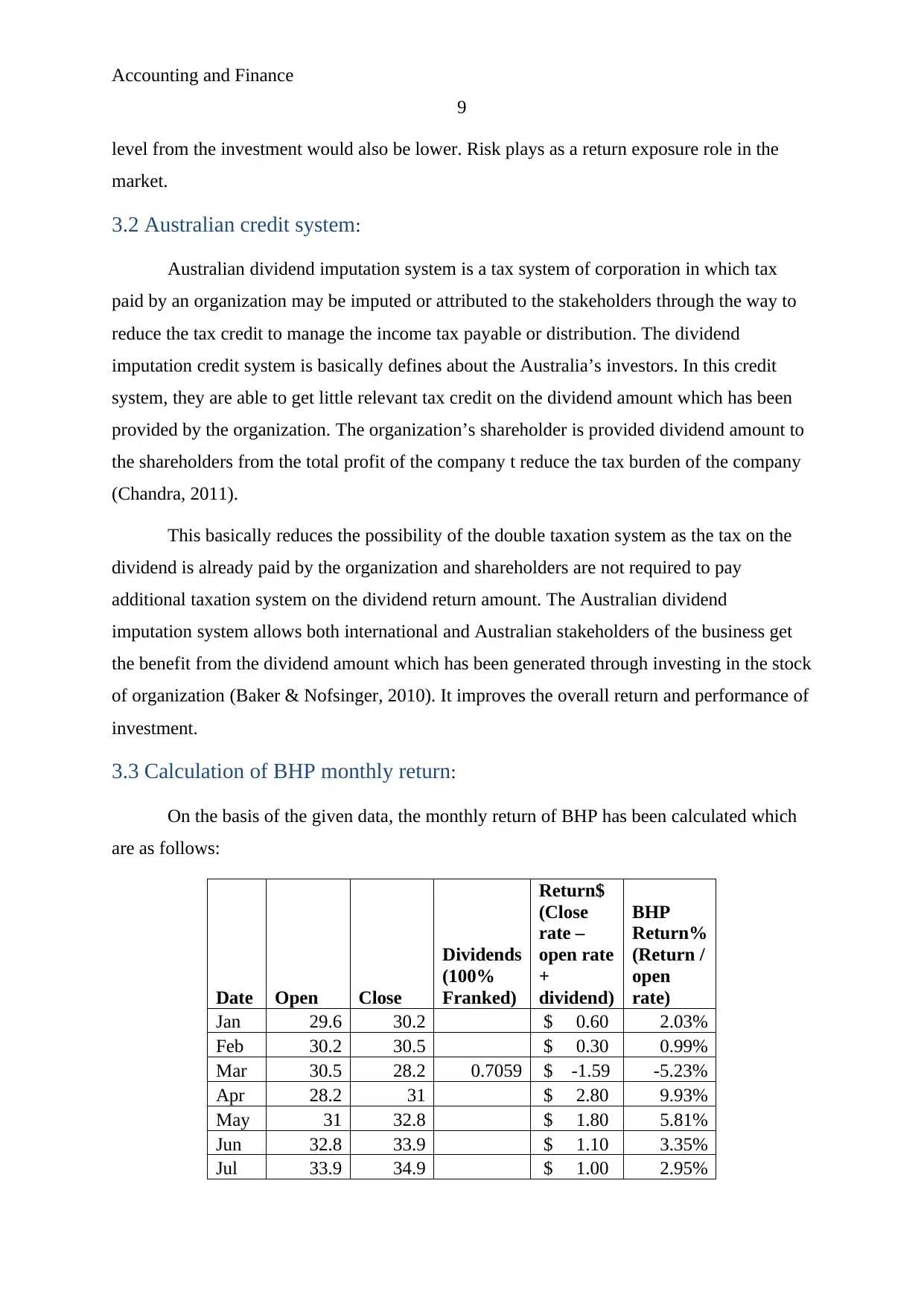
3.3 Calculation of BHP monthly return:
On the basis of the given data, the monthly return of BHP has been calculated which
are as follows:
Date Open Close
Dividends
(100%
Franked)
Return$
(Close
rate –
open rate
+
dividend)
BHP
Return%
(Return /
open
rate)
Jan 29.6 30.2 $ 0.60 2.03%
Feb 30.2 30.5 $ 0.30 0.99%
Mar 30.5 28.2 0.7059 $ -1.59 -5.23%
Apr 28.2 31 $ 2.80 9.93%
May 31 32.8 $ 1.80 5.81%
Jun 32.8 33.9 $ 1.10 3.35%
Jul 33.9 34.9 $ 1.00 2.95%

Accounting and Finance
10
Aug 34.9 33.2 $ -1.70 -4.87%
Sep 33.2 34.6 0.856 $ 2.26 6.80%
Oct 34.6 32.2 $ -2.40 -6.94%
Nov 32.2 30.7 $ -1.50 -4.66%
Dec 30.7 34.2 $ 3.50 11.40%
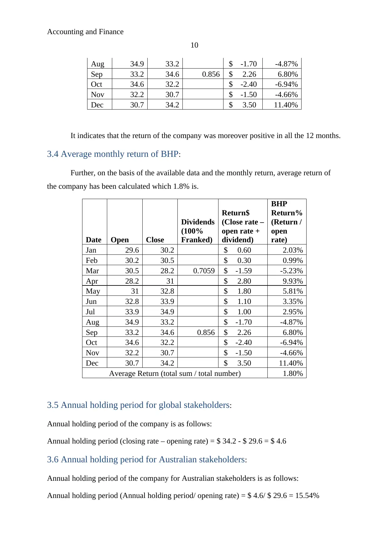
It indicates that the return of the company was moreover positive in all the 12 months.
3.4 Average monthly return of BHP:
Further, on the basis of the available data and the monthly return, average return of
the company has been calculated which 1.8% is.
Date Open Close
Dividends
(100%
Franked)
Return$
(Close rate –
open rate +
dividend)
BHP
Return%
(Return /
open
rate)
Jan 29.6 30.2 $ 0.60 2.03%
Feb 30.2 30.5 $ 0.30 0.99%
Mar 30.5 28.2 0.7059 $ -1.59 -5.23%
Apr 28.2 31 $ 2.80 9.93%
May 31 32.8 $ 1.80 5.81%
Jun 32.8 33.9 $ 1.10 3.35%
Jul 33.9 34.9 $ 1.00 2.95%
Aug 34.9 33.2 $ -1.70 -4.87%
Sep 33.2 34.6 0.856 $ 2.26 6.80%
Oct 34.6 32.2 $ -2.40 -6.94%
Nov 32.2 30.7 $ -1.50 -4.66%
Dec 30.7 34.2 $ 3.50 11.40%
Average Return (total sum / total number) 1.80%
3.5 Annual holding period for global stakeholders:
Annual holding period of the company is as follows:
Annual holding period (closing rate – opening rate) = $ 34.2 - $ 29.6 = $ 4.6
3.6 Annual holding period for Australian stakeholders:
Annual holding period of the company for Australian stakeholders is as follows:
Annual holding period (Annual holding period/ opening rate) = $ 4.6/ $ 29.6 = 15.54%

Accounting and Finance
11
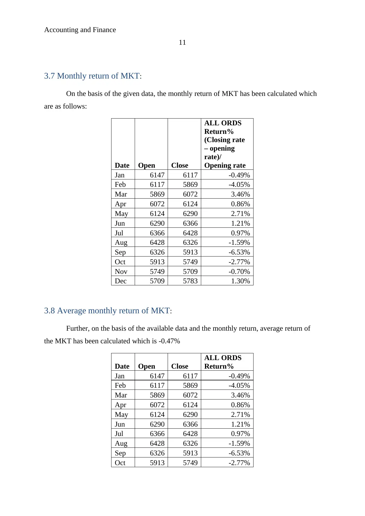
3.7 Monthly return of MKT:
On the basis of the given data, the monthly return of MKT has been calculated which
are as follows:
Date Open Close
ALL ORDS
Return%
(Closing rate
– opening
rate)/
Opening rate
Jan 6147 6117 -0.49%
Feb 6117 5869 -4.05%
Mar 5869 6072 3.46%
Apr 6072 6124 0.86%
May 6124 6290 2.71%
Jun 6290 6366 1.21%
Jul 6366 6428 0.97%
Aug 6428 6326 -1.59%
Sep 6326 5913 -6.53%
Oct 5913 5749 -2.77%
Nov 5749 5709 -0.70%
Dec 5709 5783 1.30%
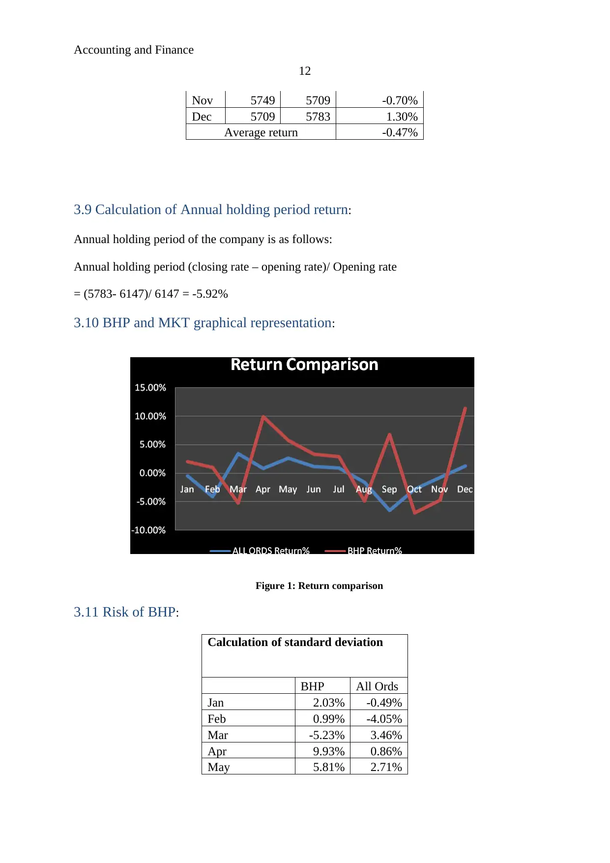
3.8 Average monthly return of MKT:
Further, on the basis of the available data and the monthly return, average return of
the MKT has been calculated which is -0.47%
Date Open Close
ALL ORDS
Return%
Jan 6147 6117 -0.49%
Feb 6117 5869 -4.05%
Mar 5869 6072 3.46%
Apr 6072 6124 0.86%
May 6124 6290 2.71%
Jun 6290 6366 1.21%
Jul 6366 6428 0.97%
Aug 6428 6326 -1.59%
Sep 6326 5913 -6.53%
Oct 5913 5749 -2.77%

Accounting and Finance
12
Nov 5749 5709 -0.70%
Dec 5709 5783 1.30%
Average return -0.47%
3.9 Calculation of Annual holding period return:
Annual holding period of the company is as follows:
Annual holding period (closing rate – opening rate)/ Opening rate
= (5783- 6147)/ 6147 = -5.92%
3.10 BHP and MKT graphical representation:
Figure 1: Return comparison
3.11 Risk of BHP:
Calculation of standard deviation
BHP All Ords
Jan 2.03% -0.49%
Feb 0.99% -4.05%
Mar -5.23% 3.46%
Apr 9.93% 0.86%
May 5.81% 2.71%

Accounting and Finance
13
Jun 3.35% 1.21%
Jul 2.95% 0.97%
Aug -4.87% -1.59%
Sep 6.80% -6.53%
Oct -6.94% -2.77%
Nov -4.66% -0.70%
Dec 11.40% 1.30%
Standard
deviation 6.15% 2.88%
It indicates that the beta of BHP and MKT is 6.15% and 2.88%. It defines that the risk
level of MKT is quite lower than the risk level of BHP.
3.12 Identifying the risk level of BHP:
On the basis of the yahoo finance, it has been found that the risk factor of BHP is
quite higher because of the beta level which is 1.12. This beta level is even higher than the
market risk of the capital market. Hence, the stock of the company has higher risk involved
for an investor which could even affect the investment portfolio of the company. Beta is
basically a measurement to identify the uncertainty level of achieving the return as per the
market and investors’ expectation. It is the extent of unexpected outcomes which are to be
realized by the investors.
Beta could be seen differently by different investors such as conservative investors would see
it as a bad factor whereas a growth investor would find it as an opportunity to earn more
return from the investment (Higgins, 2012). In the investment perspective, risk could be
considered as the return parallel from an investment. It is basically a measurement to identify
the uncertainty level of achieving the return as per the market and investors’ expectation. It is
the extent of unexpected outcomes which are to be realized by the investors. Risk attributes
could be seen differently by different investors such as conservative investors would see it as
a bad factor whereas a growth investor would find it as an opportunity to earn more return
from the investment (Higgins, 2012). In the investment perspective, risk could be considered
as the return parallel from an investment. It basically defines that the stock volatility of the
company is quite higher which would definitely affect over the return of the company.

Accounting and Finance
14
3.13 Calculation of CAPM:
CAPM is capital asset pricing model. It involves the risk free rate, market risk
premium and beta to calculate the return of investment. CAPM calculations of the company
are as follows:
Particulars Value
Rf (Risk free rate) 2.29%
Rm (Market risk premium) 9.55%
Beta 1.12
CAPM (Risk free rate + Beta * (Market risk
premium - risk free rate)) 10.42%
3.14 SML graph:
Graphical representation of CAPM calculations of the company are as follows:
Figure 2: Security Market Line
3.15 SML graph (BHP and MKT):
The graph of SML is as follows after considering the actual return of 2018 of the
company:

Accounting and Finance
15
Figure 3: security market line 1
3.16 Portfolio’s return and beta:
On the basis of the available data of BHP and All ords, a portfolio has been created.
The risk and return of that portfolio has been given as follows:
Particulars BHP ALL ords
Return 10.42% 9.55%
Beta 1.12 1
Weight 40% 60%
Portfolio return
(40%*10.42%) +
(60%*9.55%) 9.90%
Portfolio beta
(40%*1.12)+(60%*1) 1.05
On the basis of the above result, it has been considered that the portfolio risk and
portfolio return of the company is 9.90% and 1.05. It defines that the risk level of portfolio is
quite lesser. However, it is higher than the market risk whereas the portfolio return of the
investment is also higher. To conclude, the portfolio choice of the company is quite better.

Accounting and Finance
16
References:
Baker, H.K. & Nofsinger, J.R. (2010). Behavioral Finance: Investors, Corporations, &
Markets. UK: John Wiley & Sons.
Chandra, P. (2011). Financial management. Tata McGraw-Hill Education.
Elton, E.J., Gruber, M.J., Brown, S.J., & Goetzmann, W.N. (2009). Modern Portfolio Theory
& Investment Analysis. UK: John Wiley & Sons.
Higgins, R. C. (2012). Analysis for marketing management. McGraw-Hill/Irwin.
Madura, J. (2014). Financial Markets & Institutions. US: Cengage Learning.
Palicka, V.J. (2011). Fusion Analysis: Merging Fundamental & Technical Analysis for Risk-
Adjusted Excess Returns. McGraw Hill Professional.
Rabin, M. (2013). Risk aversion and expected-utility theory: A calibration theorem.
In Handbook of the Fundamentals of Financial Decision Making: Part I (pp. 241-252).
Rose, P. S., & Hudgins, S. C. (2012). Bank management & financial services. McGraw-Hill
Education.
Schlichting, T. (2013). Fundamental Analysis, Behavioral Finance & Technical Analysis on
the Stock Market. GRIN Verlag.