Accounting Decision Support Tools Assignment

Accounting Decision Support Tools
Assignment –III
Student Name
[Pick the date]

Question 1
(a) Steps that need to be undertaken as part of decision making are briefly highlighted below.
 The decision maker needs to objectively outline the decision expectations along with
the outcomes that are possible for the given decision.
 The decision maker would be presented with various possible alternatives that need to
be identified.
 The indiviual analysis of the alternative needs to be undetaken considering the
potential outcomes and their respective likelihood.
 For the host of outcoems that have been identified , a payoff matrix needs to be
created keeping the risk into consideration.
 Considering the payooff matrix derived in the above step, the decision maker should
apply the selected decision making model for making the final decision.
(b) Alternatives are the varying strategies that are available for deployment by the decision
maker in wake of the underlying decision. However, these alternatives are linked to the states
of nature which are potential future events which cannot be controlled by the decision maker.
For different states of nature, the alternative would vary but the challenge for the decision
maker is to pick an alternative which is suitable considering the likely future states.
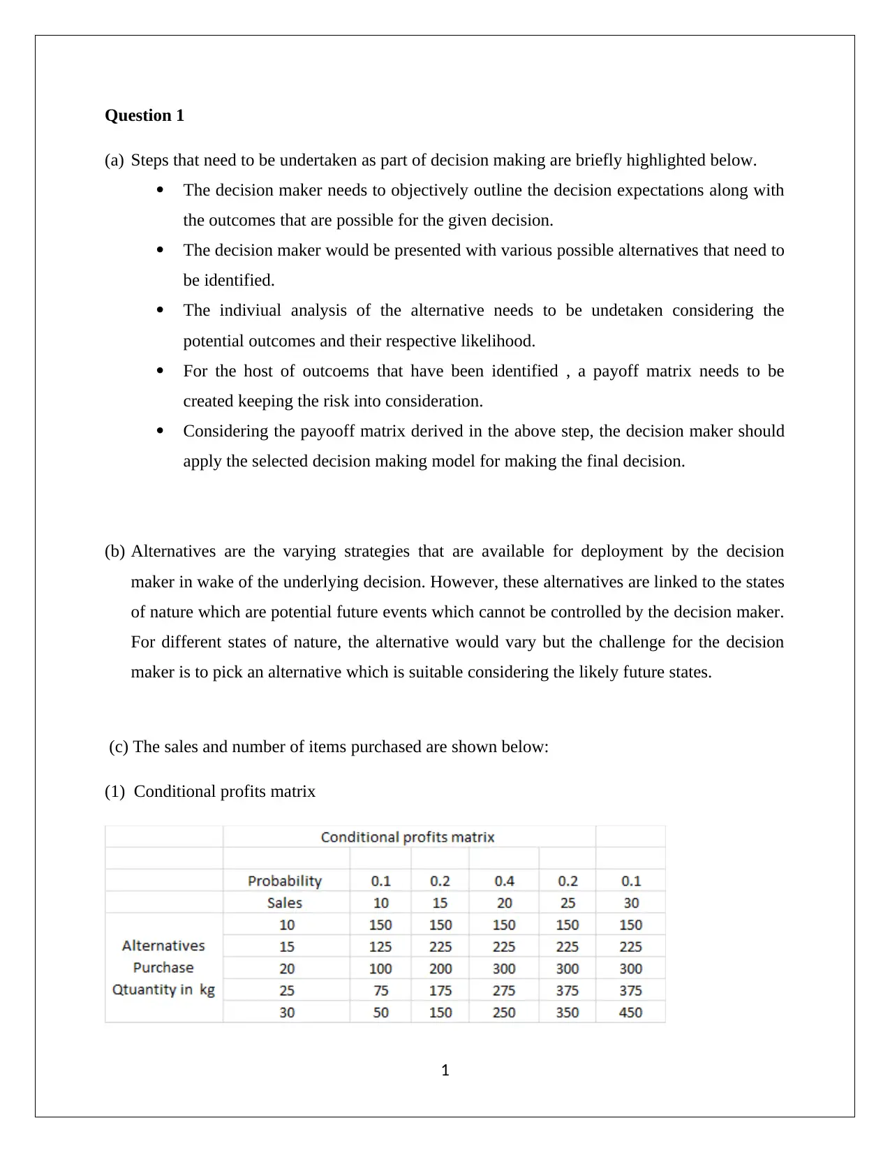
(c) The sales and number of items purchased are shown below:
(1) Conditional profits matrix
1

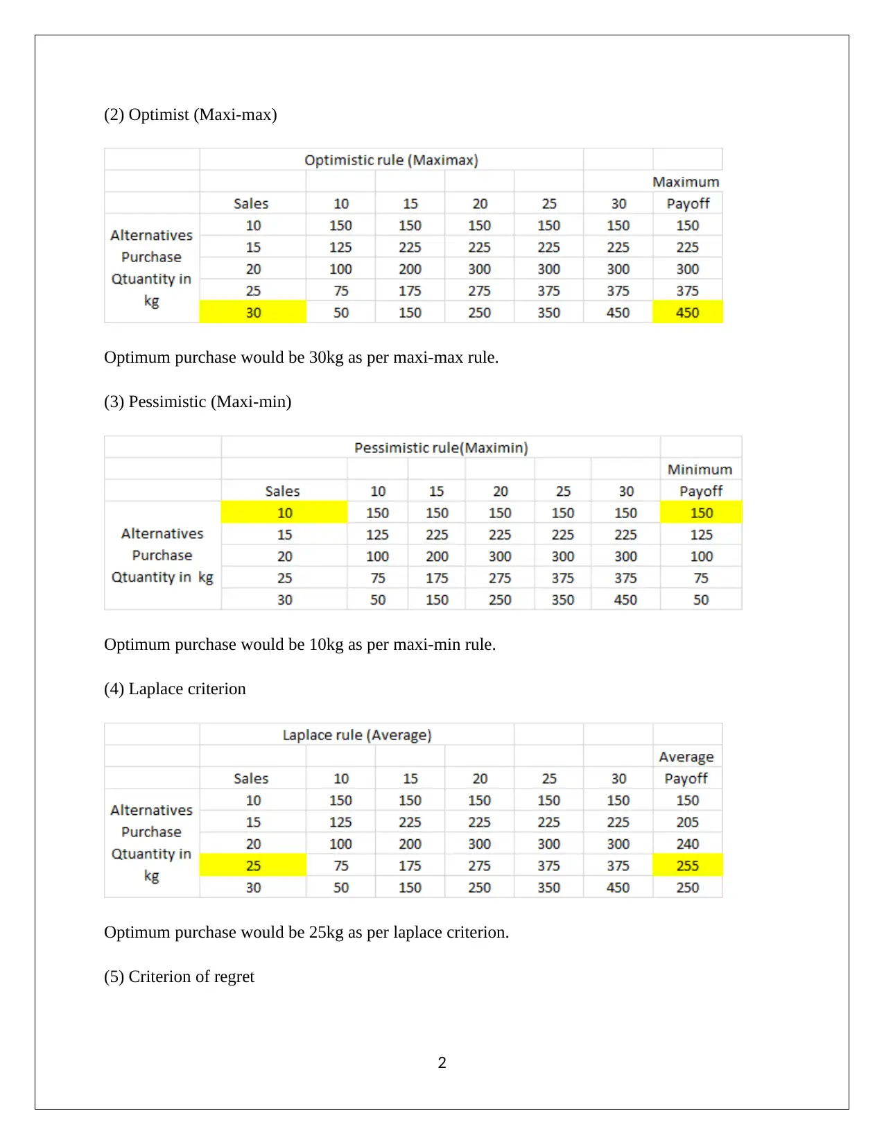
(2) Optimist (Maxi-max)
Optimum purchase would be 30kg as per maxi-max rule.
(3) Pessimistic (Maxi-min)
Optimum purchase would be 10kg as per maxi-min rule.
(4) Laplace criterion
Optimum purchase would be 25kg as per laplace criterion.
(5) Criterion of regret
2

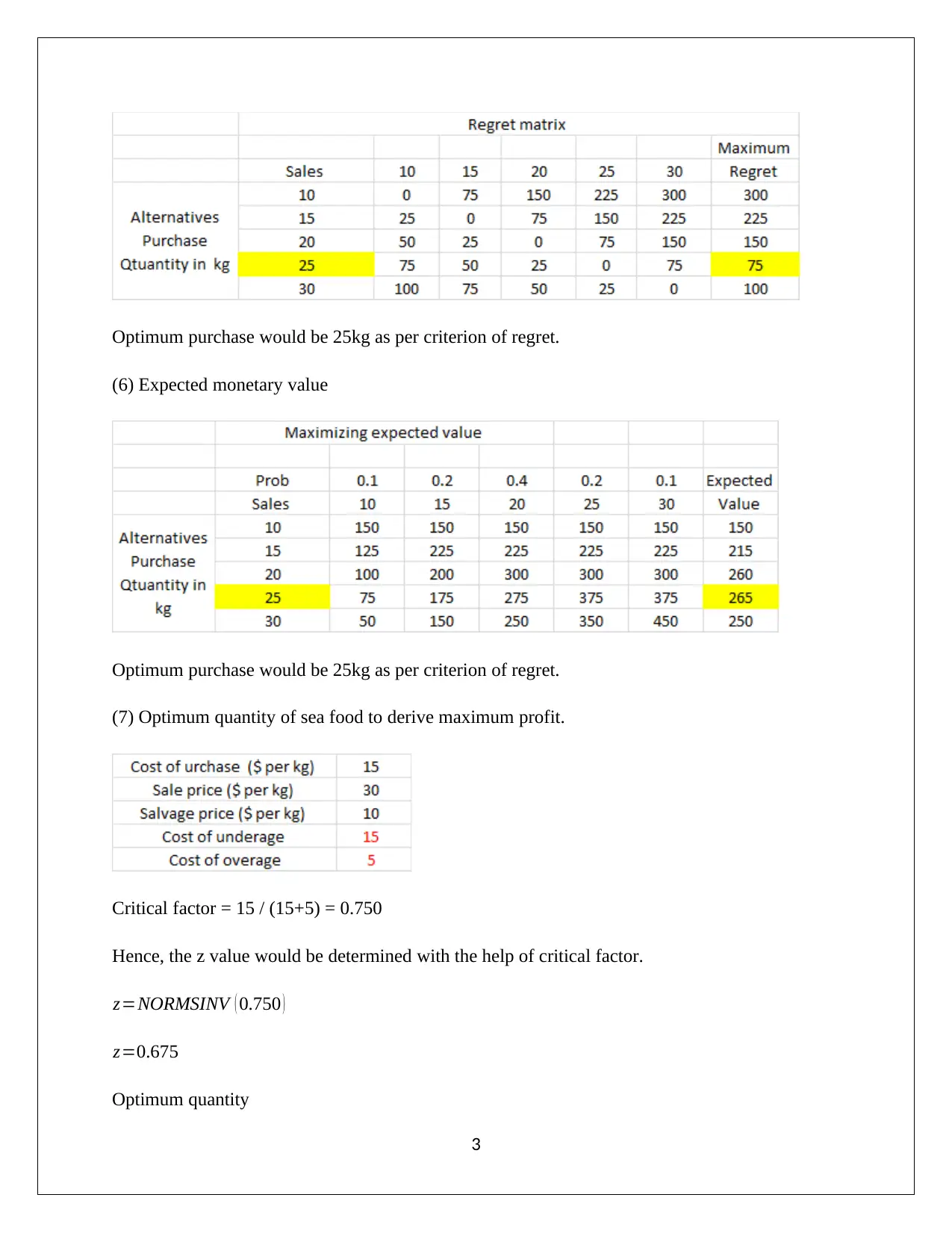
Optimum purchase would be 25kg as per criterion of regret.
(6) Expected monetary value
Optimum purchase would be 25kg as per criterion of regret.
(7) Optimum quantity of sea food to derive maximum profit.
Critical factor = 15 / (15+5) = 0.750
Hence, the z value would be determined with the help of critical factor.
z=NORMSINV ( 0.750 )
z=0.675
Optimum quantity
3

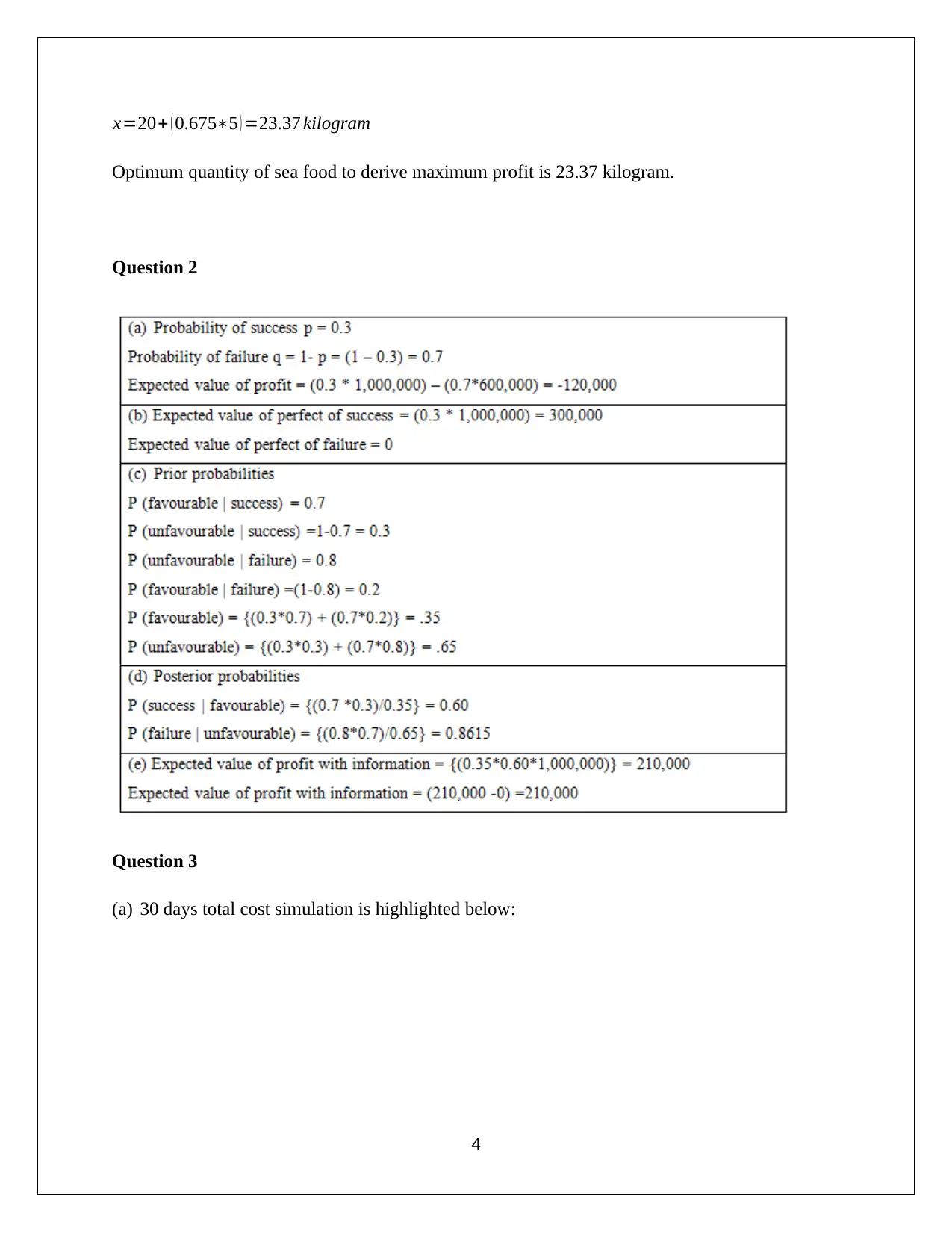
x=20+ ( 0.675∗5 ) =23.37 kilogram
Optimum quantity of sea food to derive maximum profit is 23.37 kilogram.
Question 2
Question 3
(a) 30 days total cost simulation is highlighted below:
4

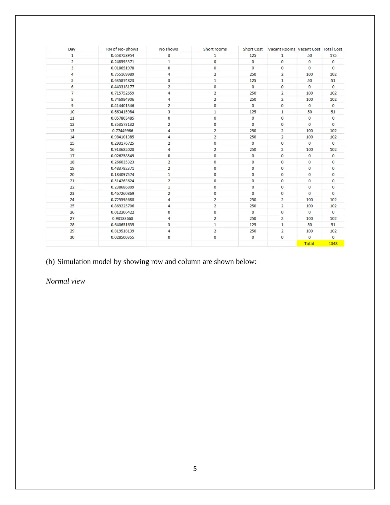
(b) Simulation model by showing row and column are shown below:
Normal view
5

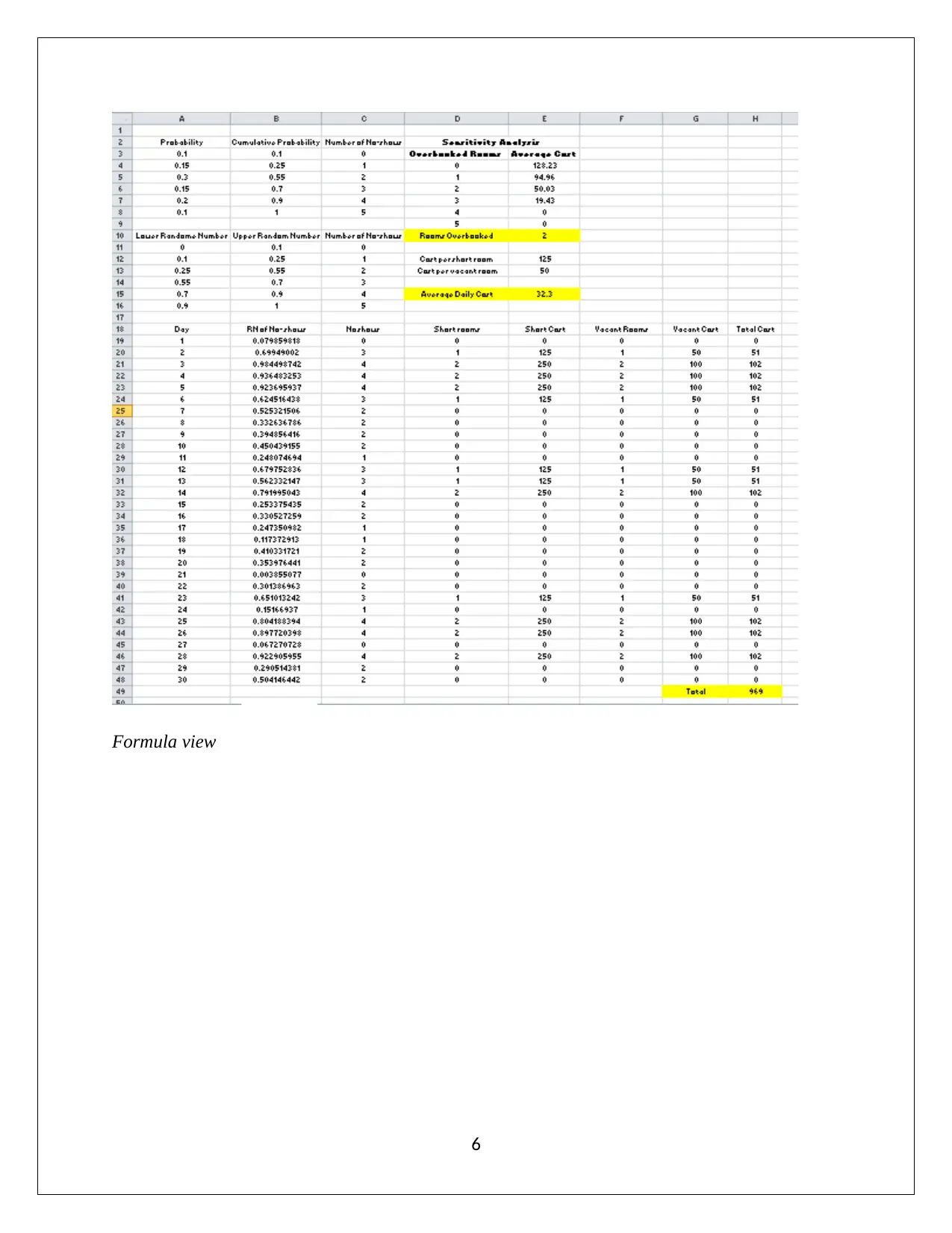
Formula view
6

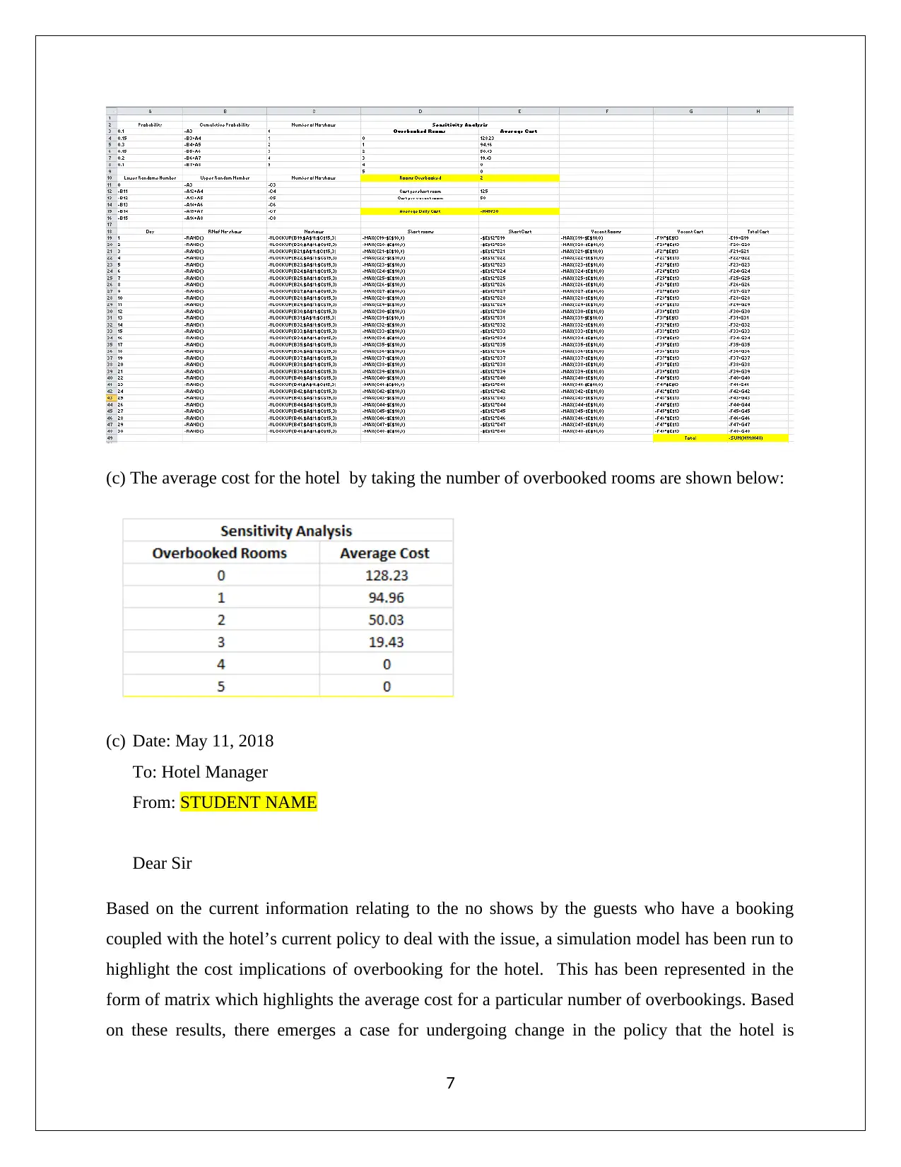
(c) The average cost for the hotel by taking the number of overbooked rooms are shown below:
(c) Date: May 11, 2018
To: Hotel Manager
From: STUDENT NAME
Dear Sir
Based on the current information relating to the no shows by the guests who have a booking
coupled with the hotel’s current policy to deal with the issue, a simulation model has been run to
highlight the cost implications of overbooking for the hotel. This has been represented in the
form of matrix which highlights the average cost for a particular number of overbookings. Based
on these results, there emerges a case for undergoing change in the policy that the hotel is
7

currently following since by enhancing the overbookings to four, the average cost can further
come down.
Question 4
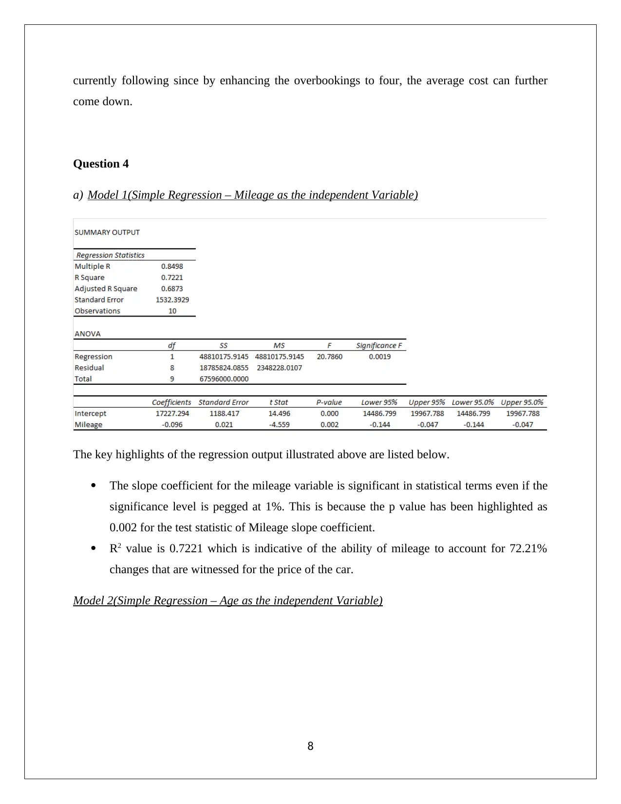
a) Model 1(Simple Regression – Mileage as the independent Variable)
The key highlights of the regression output illustrated above are listed below.
 The slope coefficient for the mileage variable is significant in statistical terms even if the
significance level is pegged at 1%. This is because the p value has been highlighted as
0.002 for the test statistic of Mileage slope coefficient.
 R2 value is 0.7221 which is indicative of the ability of mileage to account for 72.21%
changes that are witnessed for the price of the car.
Model 2(Simple Regression – Age as the independent Variable)
8

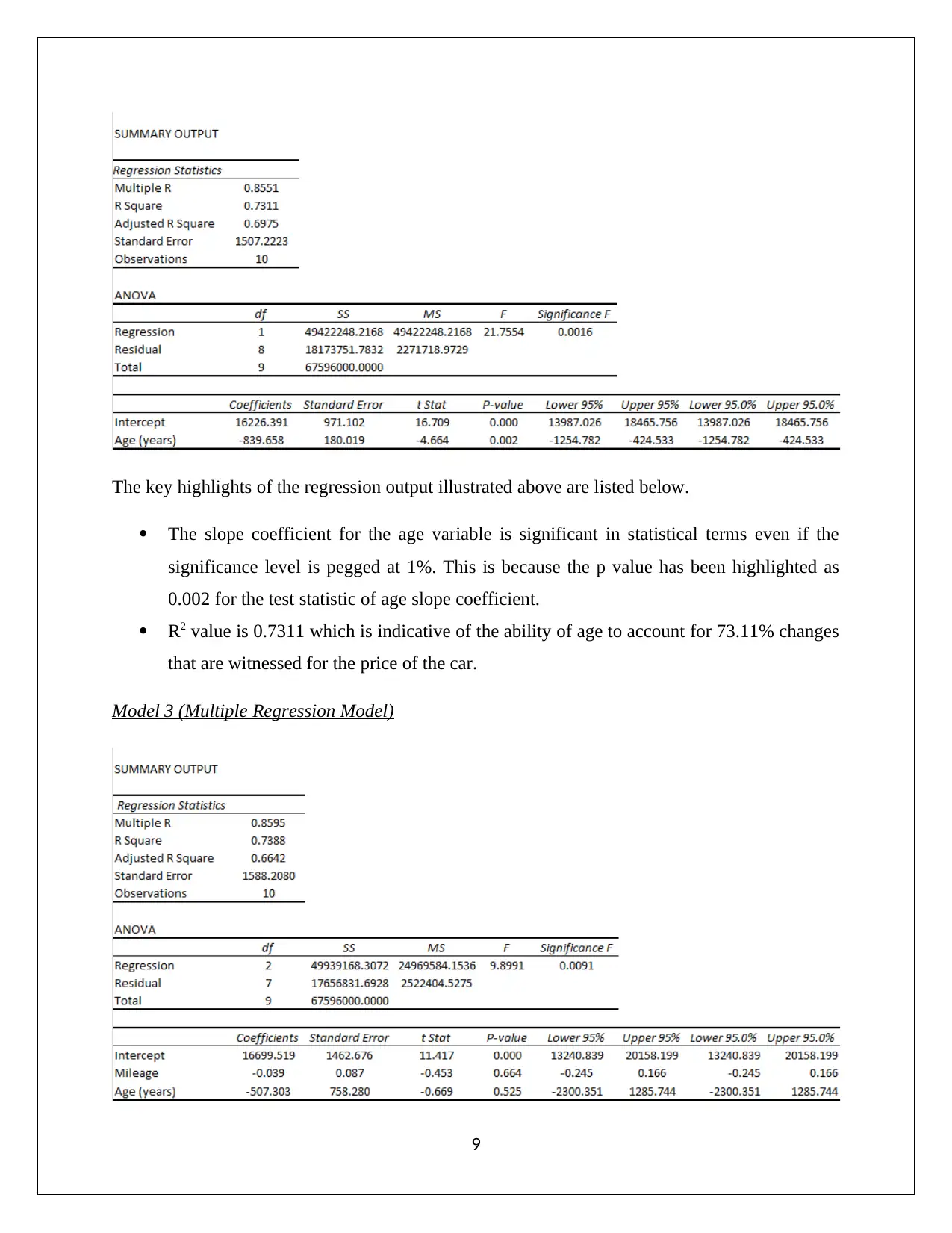
The key highlights of the regression output illustrated above are listed below.
 The slope coefficient for the age variable is significant in statistical terms even if the
significance level is pegged at 1%. This is because the p value has been highlighted as
0.002 for the test statistic of age slope coefficient.
 R2 value is 0.7311 which is indicative of the ability of age to account for 73.11% changes
that are witnessed for the price of the car.
Model 3 (Multiple Regression Model)
9

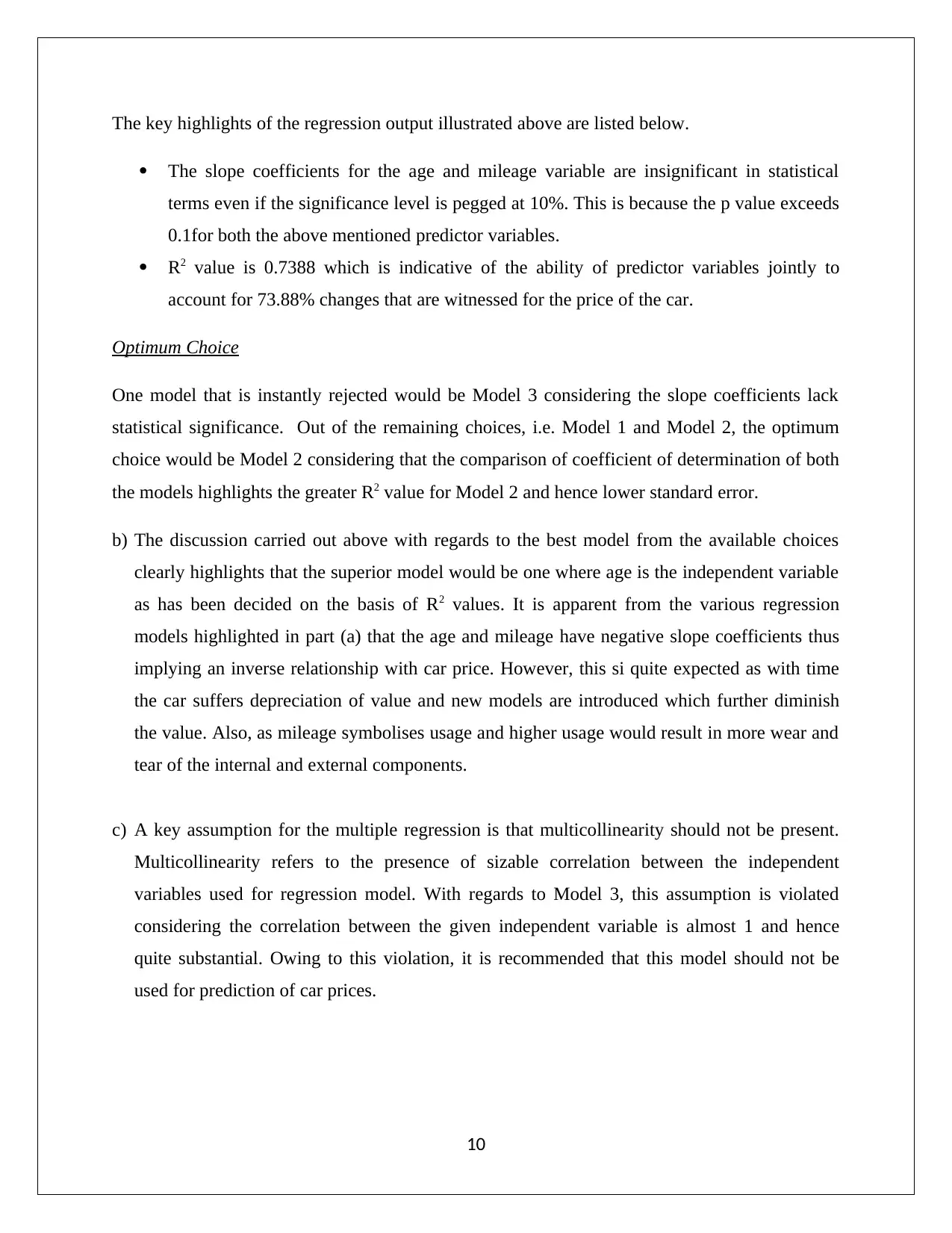
The key highlights of the regression output illustrated above are listed below.
 The slope coefficients for the age and mileage variable are insignificant in statistical
terms even if the significance level is pegged at 10%. This is because the p value exceeds
0.1for both the above mentioned predictor variables.
 R2 value is 0.7388 which is indicative of the ability of predictor variables jointly to
account for 73.88% changes that are witnessed for the price of the car.
Optimum Choice
One model that is instantly rejected would be Model 3 considering the slope coefficients lack
statistical significance. Out of the remaining choices, i.e. Model 1 and Model 2, the optimum
choice would be Model 2 considering that the comparison of coefficient of determination of both
the models highlights the greater R2 value for Model 2 and hence lower standard error.
b) The discussion carried out above with regards to the best model from the available choices
clearly highlights that the superior model would be one where age is the independent variable
as has been decided on the basis of R2 values. It is apparent from the various regression
models highlighted in part (a) that the age and mileage have negative slope coefficients thus
implying an inverse relationship with car price. However, this si quite expected as with time
the car suffers depreciation of value and new models are introduced which further diminish
the value. Also, as mileage symbolises usage and higher usage would result in more wear and
tear of the internal and external components.
c) A key assumption for the multiple regression is that multicollinearity should not be present.
Multicollinearity refers to the presence of sizable correlation between the independent
variables used for regression model. With regards to Model 3, this assumption is violated
considering the correlation between the given independent variable is almost 1 and hence
quite substantial. Owing to this violation, it is recommended that this model should not be
used for prediction of car prices.
10

Question 5
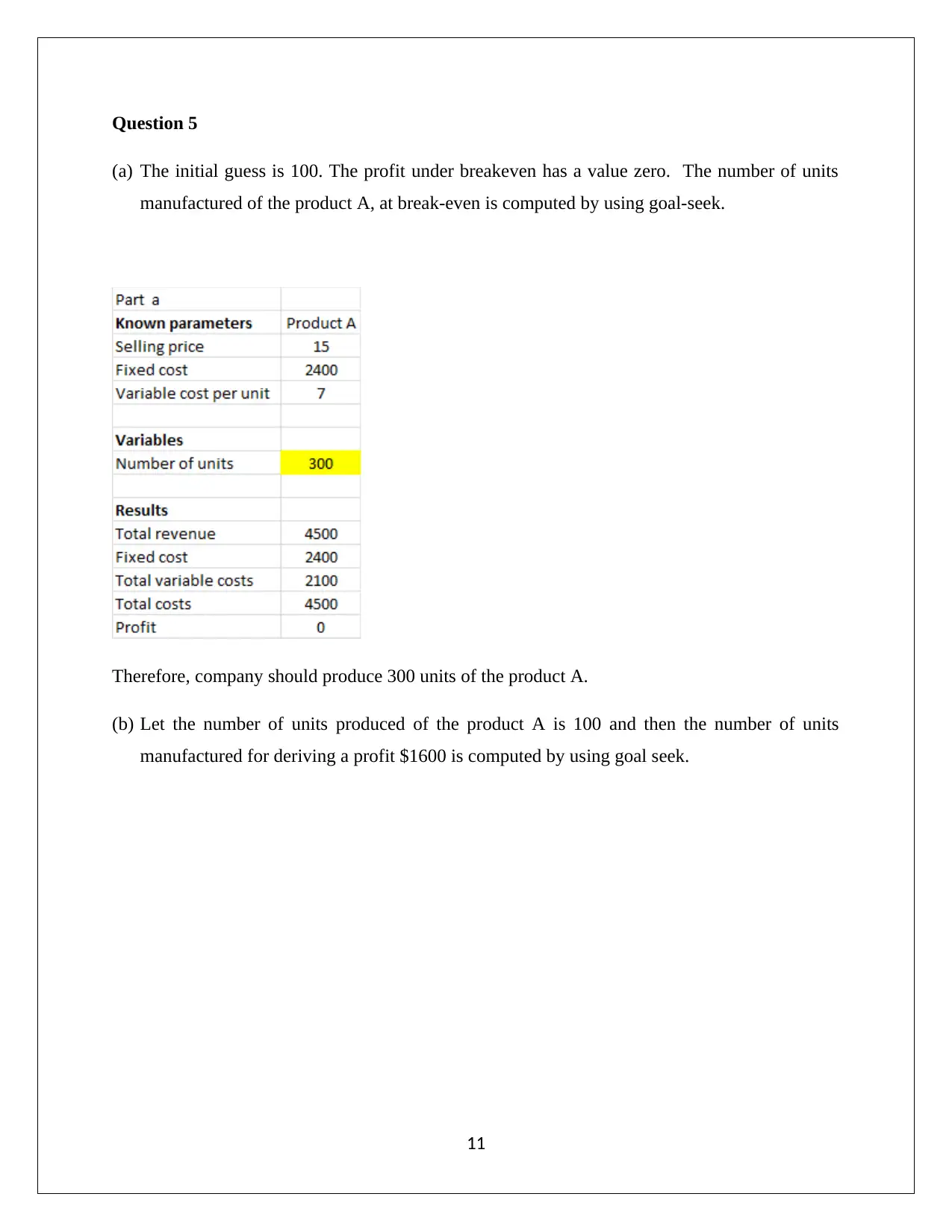
(a) The initial guess is 100. The profit under breakeven has a value zero. The number of units
manufactured of the product A, at break-even is computed by using goal-seek.
Therefore, company should produce 300 units of the product A.
(b) Let the number of units produced of the product A is 100 and then the number of units
manufactured for deriving a profit $1600 is computed by using goal seek.
11

Therefore, company should manufacture 500 units of the product A for deriving a profit of
$1600.
(c) The ratio of producing product A and product B is 2:1. Hence, let the unit manufactured for
product B is x and units produced for product A is 2x.
Let the initial guess for producing product B is 100. After using goal-seek the optimum values
for product A and B are computed and is shown below:
12

Hence, the optimum production units for product A and B is 2000 and 1000 respectively.
13