Analytic Capability of Different Issues Using Python & R PDF

Advance Analytic Capability of Different Issues Using Python & R
STUDENT NAME:
STUDENT ID:
1

Table of Contents
Introduction......................................................................................................................................2
Python..............................................................................................................................................2
R.......................................................................................................................................................4
Machine Learning............................................................................................................................5
Analytical tool.................................................................................................................................5
Association....................................................................................................................................12
Correlation.....................................................................................................................................20
Regression......................................................................................................................................23
Clustering.......................................................................................................................................25
Anomaly Detection........................................................................................................................30
Reference list.................................................................................................................................35

Introduction
In recent era of development, we face different challenges related to automotive structure of
systems. As our world undergoes in very fast pace, each and every objective and work needs
perfection but human it barely performs such. So they go for programming and algorithm for
doing such. In our everyday life, we see several intelligent applications in out computers and
mobiles which include automated assistance, speech recognizer, face recognizer, map assistance
and route director, product assistance, product comparison analyzer and many more (Dincer et
al. 2017). We live in our world to make it beautiful and those are the inevitable requirements.
Those applications are done using different programming languages as per the ability to write
code and all.
Intelligent application or more specifically, Artificial Intelligence applications require something
more than the conservative programming architecture. Thus, we have to choose such languages
which meetthese criteria. Lots of Languages are available for this purpose like C, C++, Java,
Python, Matlab, Ruby, PHP, R etc. Those have their separate library structure and different
procedures. For AI applications, we should choose such languages which have enough rich
library and wide variety of coding structure and should be human friendly. Thus much of the
majority chose Python and R for this purpose (Volk et al. 2017).
Now first we see the features of those in a comparative manner.
Python
Python was developed and introduced by Guido Van Rossum in 1991. It has rich backbone of
C++. Python is a exclusive Object Oriented Language specially used for Scientific and Analytic
purpose. Data visualization is very easy in Python and so that if data analysis and visualization
comes in the scenario, we can perform such task using Python.
 Features

The important features and advantages of Python are (Antony et al. 2017):
1. Python is Dynamically Typed Language means it does not require any variable to be
assigned with its type rather those variable types are dynamically allocated.
2. Python is Interpreted Language.
3. The coding execution is very easy in Python
4. Easy to read the codes and syntaxes.
5. It is very expressive language as the syntax and codes are used mostly based on English
meaningful phrases.
6. Python is an Open-Source Language and all the packages need to be incorporated also
they are open sources.
7. This is a High Level OOP Language.
8. It supports portability that is once you have written any code in any OS, this code can be
run in any other platform or OS.
9. It has an extensible facility of merging and transforming code to different languages like
C, MATLAB etc.
10. Python code support embedding into device for example Micro Python, Raspberry Pi.
11. It has large standard library.
12. GUI programming is much easier.
 Applications:
Python is applicable in many areas like:
 Numerical Computation
 Scientific Computation
 Machine Learning
 Data Science
 Data Mining
 Web Development
 Artificial Intelligence.

R
Another programming language of interest is R. R is basically and widely used for scientific and
Statistical computations. It has a facility to have one of the richest libraries among all the
languages (Nelson, 2016). As for the richness and wide availability, many of the data scientists
and scientist of machine learning prefer R. R was introduced by Ross Ihaka and Robert
Gentleman in 1993.
 Features
The features of R are:
1. This is a well-developed, simple and effective programming language.
2. It has an effective data handling and storage facility,
3. It provides a range of operators for calculations on arrays, lists, vectors and matrices.
4. It provides a large, coherent and integrated collection of tools for data analysis.
5. It provides GUI facility.
 Applications
R is applicable in many different areas like:
 Data Analysis
 Case matching
 Statistical Analysis
 Online data mining
 Face and Tag detection
 Data Science
 Machine Learning
 Artificial Intelligence

Let we discuss about one of applications which can be done using both Python and R. One of the
most demanding and hot topic for now a days is Machine Learning.
Machine Learning
Machine Learning is a set of algorithms with which the programmer will assign some objective
and which tends to learn the algorithm as per the requirement. Here program is not done
explicitly rather the algorithm is made such that it capable of learning from the environment with
being explicit definition of each cases (Prakash, 2015).
Machine Learning uses different integration of issues like data, algorithm analysis tool and a
platform to execute these. When the part of analysis comes into the scenario, it is inevitable to
use the statistics. Statistics helps the algorithm to analyze data is depth with application of
statistical calculations.
Here we will make the comparative discussion on the following topics with analysis and
simulation based on both Python & R. The topics are:
 Analytic tool
 Classification
 Association
 Correlation
 Regression
 Clustering
 Anomaly Detection
Analytical tool
Analytical tool stands for the analysis on a given data. The dataset is provided and we have to
analysis these with Python & R and have again to compare.

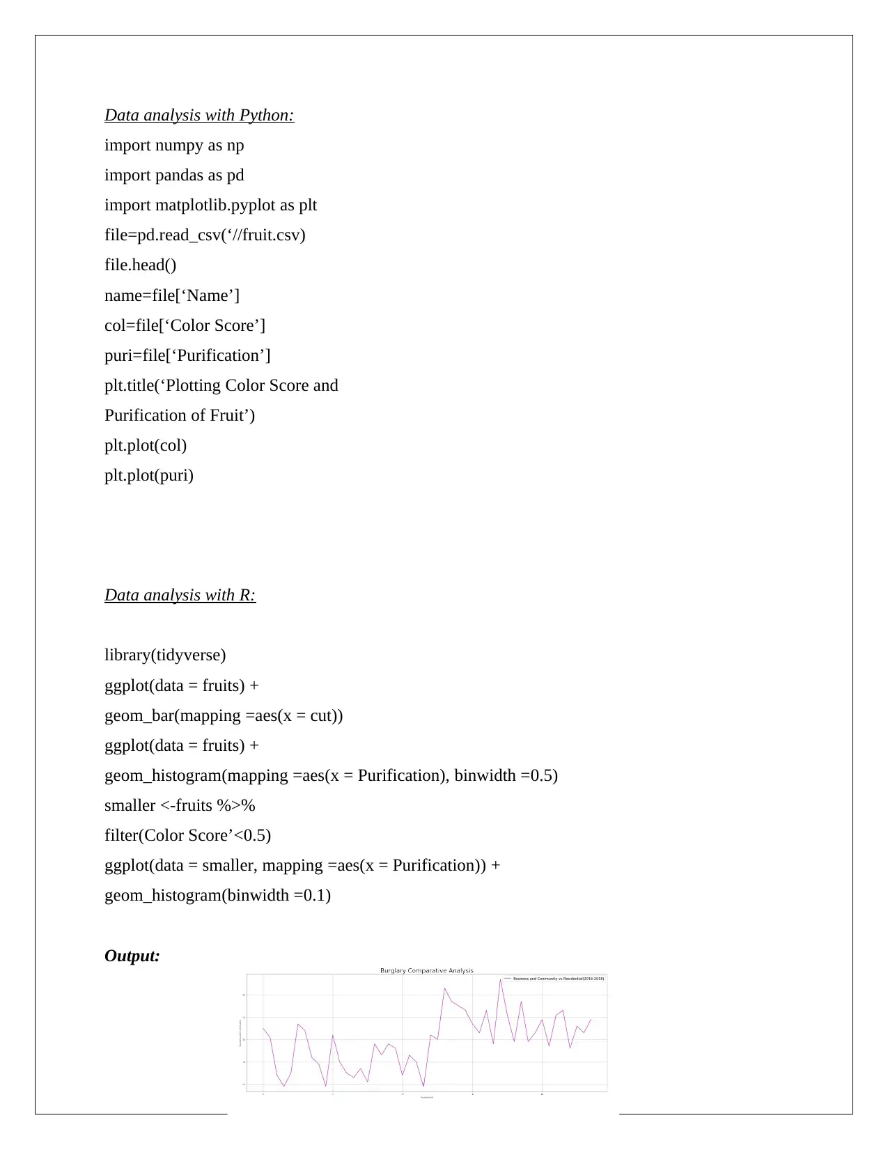
Data analysis with Python:
import numpy as np
import pandas as pd
import matplotlib.pyplot as plt
file=pd.read_csv(‘//fruit.csv)
file.head()
name=file[‘Name’]
col=file[‘Color Score’]
puri=file[‘Purification’]
plt.title(‘Plotting Color Score and
Purification of Fruit’)
plt.plot(col)
plt.plot(puri)
Data analysis with R:
library(tidyverse)
ggplot(data = fruits) +
geom_bar(mapping =aes(x = cut))
ggplot(data = fruits) +
geom_histogram(mapping =aes(x = Purification), binwidth =0.5)
smaller <-fruits %>%
filter(Color Score’<0.5)
ggplot(data = smaller, mapping =aes(x = Purification)) +
geom_histogram(binwidth =0.1)
Output:

Comparative Discussion:
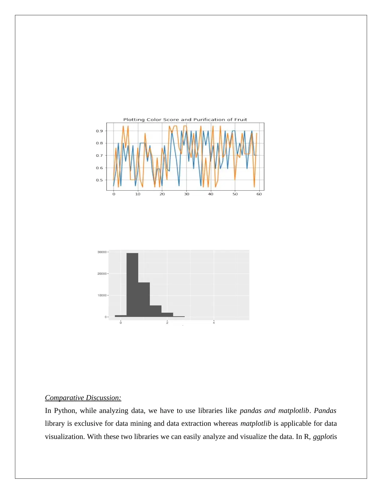
In Python, while analyzing data, we have to use libraries like pandas and matplotlib. Pandas
library is exclusive for data mining and data extraction whereas matplotlib is applicable for data
visualization. With these two libraries we can easily analyze and visualize the data. In R, ggplotis

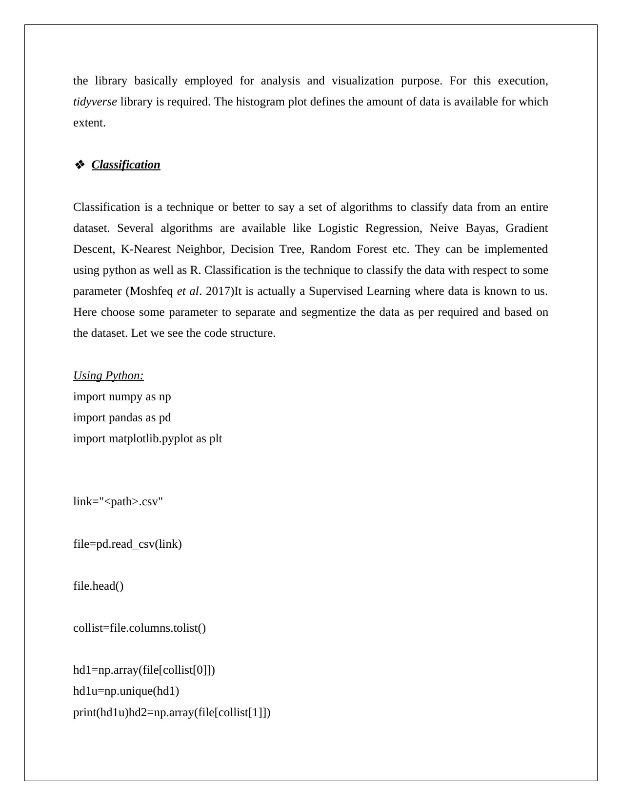
the library basically employed for analysis and visualization purpose. For this execution,
tidyverse library is required. The histogram plot defines the amount of data is available for which
extent.
 Classification
Classification is a technique or better to say a set of algorithms to classify data from an entire
dataset. Several algorithms are available like Logistic Regression, Neive Bayas, Gradient
Descent, K-Nearest Neighbor, Decision Tree, Random Forest etc. They can be implemented
using python as well as R. Classification is the technique to classify the data with respect to some
parameter (Moshfeq et al. 2017)It is actually a Supervised Learning where data is known to us.
Here choose some parameter to separate and segmentize the data as per required and based on
the dataset. Let we see the code structure.
Using Python:
import numpy as np
import pandas as pd
import matplotlib.pyplot as plt
link="<path>.csv"
file=pd.read_csv(link)
file.head()
collist=file.columns.tolist()
hd1=np.array(file[collist[0]])
hd1u=np.unique(hd1)
print(hd1u)hd2=np.array(file[collist[1]])

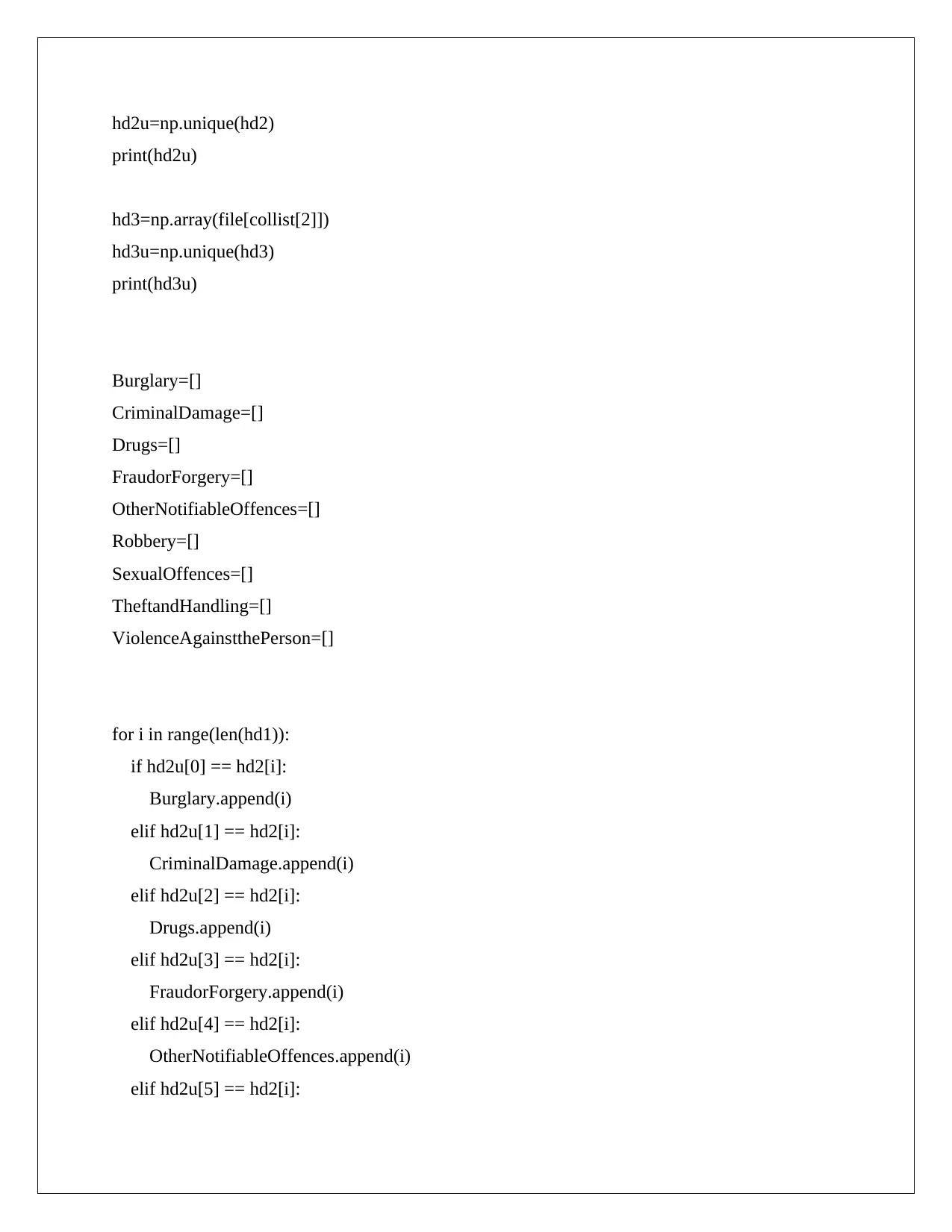
hd2u=np.unique(hd2)
print(hd2u)
hd3=np.array(file[collist[2]])
hd3u=np.unique(hd3)
print(hd3u)
Burglary=[]
CriminalDamage=[]
Drugs=[]
FraudorForgery=[]
OtherNotifiableOffences=[]
Robbery=[]
SexualOffences=[]
TheftandHandling=[]
ViolenceAgainstthePerson=[]
for i in range(len(hd1)):
if hd2u[0] == hd2[i]:
Burglary.append(i)
elif hd2u[1] == hd2[i]:
CriminalDamage.append(i)
elif hd2u[2] == hd2[i]:
Drugs.append(i)
elif hd2u[3] == hd2[i]:
FraudorForgery.append(i)
elif hd2u[4] == hd2[i]:
OtherNotifiableOffences.append(i)
elif hd2u[5] == hd2[i]:

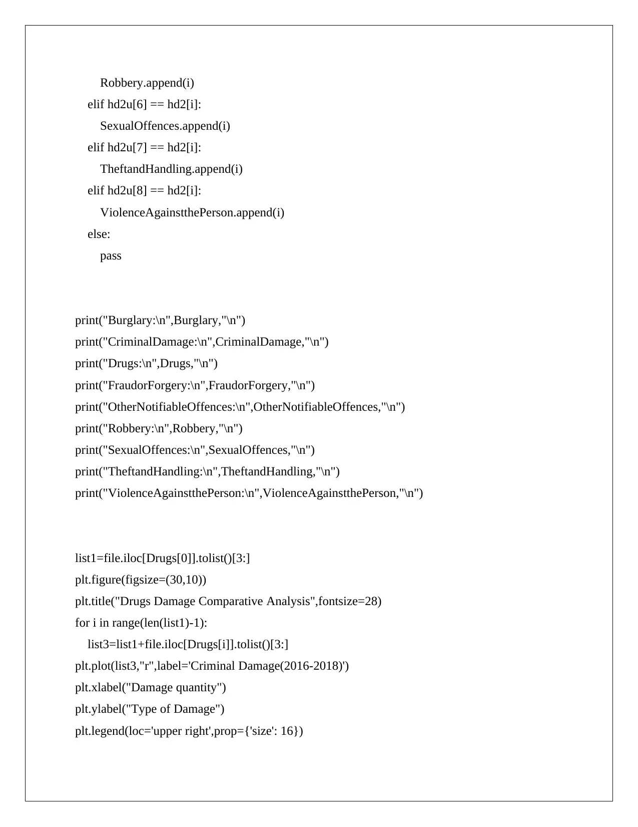
Robbery.append(i)
elif hd2u[6] == hd2[i]:
SexualOffences.append(i)
elif hd2u[7] == hd2[i]:
TheftandHandling.append(i)
elif hd2u[8] == hd2[i]:
ViolenceAgainstthePerson.append(i)
else:
pass
print("Burglary:\n",Burglary,"\n")
print("CriminalDamage:\n",CriminalDamage,"\n")
print("Drugs:\n",Drugs,"\n")
print("FraudorForgery:\n",FraudorForgery,"\n")
print("OtherNotifiableOffences:\n",OtherNotifiableOffences,"\n")
print("Robbery:\n",Robbery,"\n")
print("SexualOffences:\n",SexualOffences,"\n")
print("TheftandHandling:\n",TheftandHandling,"\n")
print("ViolenceAgainstthePerson:\n",ViolenceAgainstthePerson,"\n")
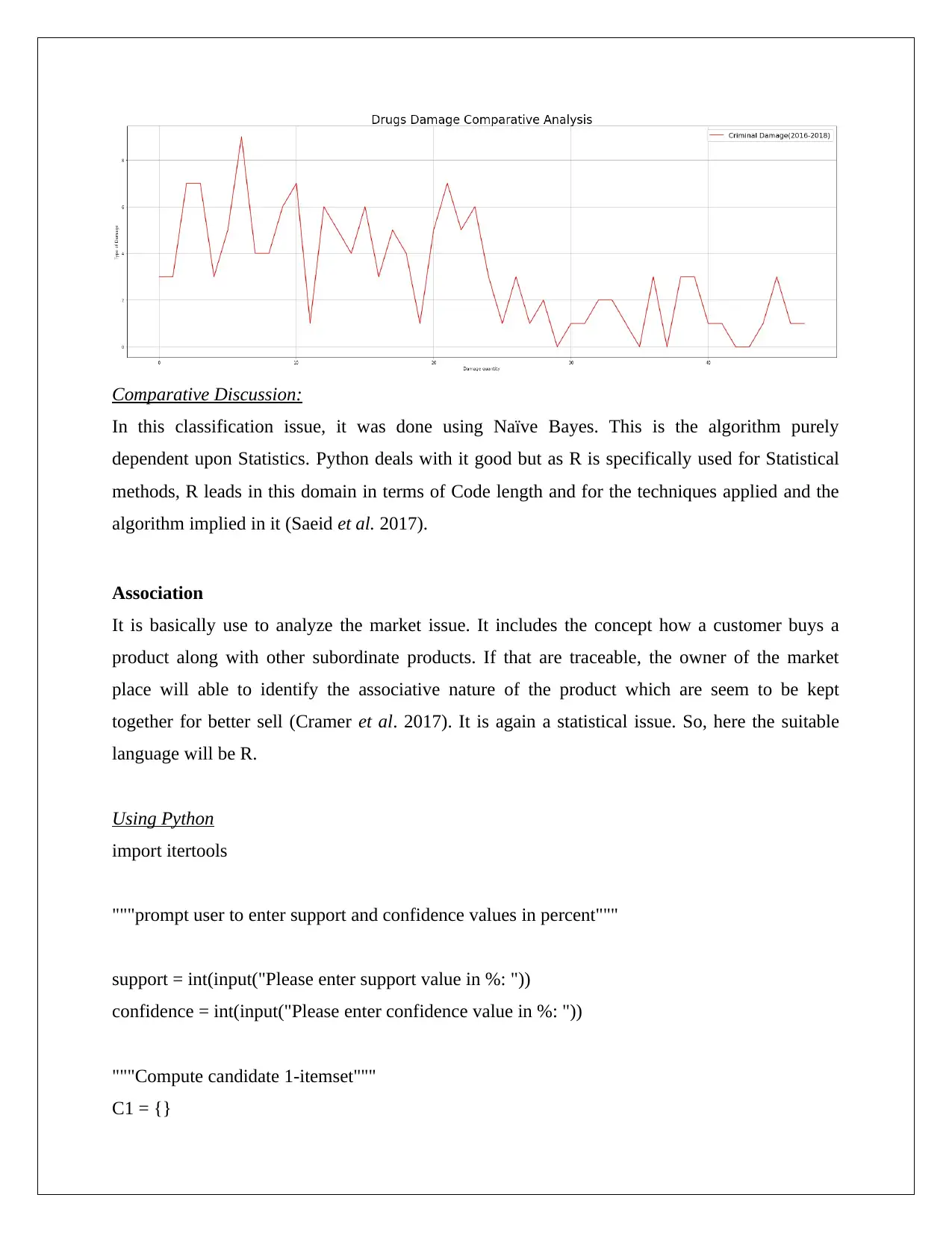
list1=file.iloc[Drugs[0]].tolist()[3:]
plt.figure(figsize=(30,10))
plt.title("Drugs Damage Comparative Analysis",fontsize=28)
for i in range(len(list1)-1):
list3=list1+file.iloc[Drugs[i]].tolist()[3:]
plt.plot(list3,"r",label='Criminal Damage(2016-2018)')
plt.xlabel("Damage quantity")
plt.ylabel("Type of Damage")
plt.legend(loc='upper right',prop={'size': 16})

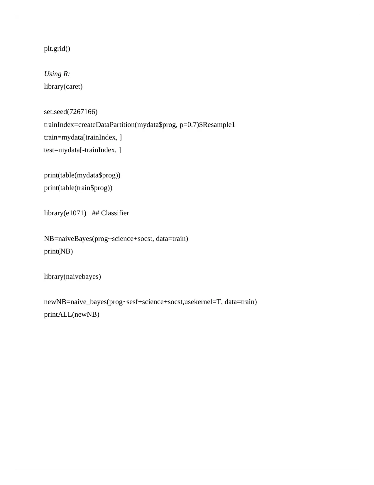
plt.grid()
Using R:
library(caret)
set.seed(7267166)
trainIndex=createDataPartition(mydata$prog, p=0.7)$Resample1
train=mydata[trainIndex, ]
test=mydata[-trainIndex, ]
print(table(mydata$prog))
print(table(train$prog))
library(e1071) ## Classifier
NB=naiveBayes(prog~science+socst, data=train)
print(NB)
library(naivebayes)
newNB=naive_bayes(prog~sesf+science+socst,usekernel=T, data=train)
printALL(newNB)

Comparative Discussion:
In this classification issue, it was done using Naïve Bayes. This is the algorithm purely
dependent upon Statistics. Python deals with it good but as R is specifically used for Statistical
methods, R leads in this domain in terms of Code length and for the techniques applied and the
algorithm implied in it (Saeid et al. 2017).
Association
It is basically use to analyze the market issue. It includes the concept how a customer buys a
product along with other subordinate products. If that are traceable, the owner of the market
place will able to identify the associative nature of the product which are seem to be kept
together for better sell (Cramer et al. 2017). It is again a statistical issue. So, here the suitable
language will be R.
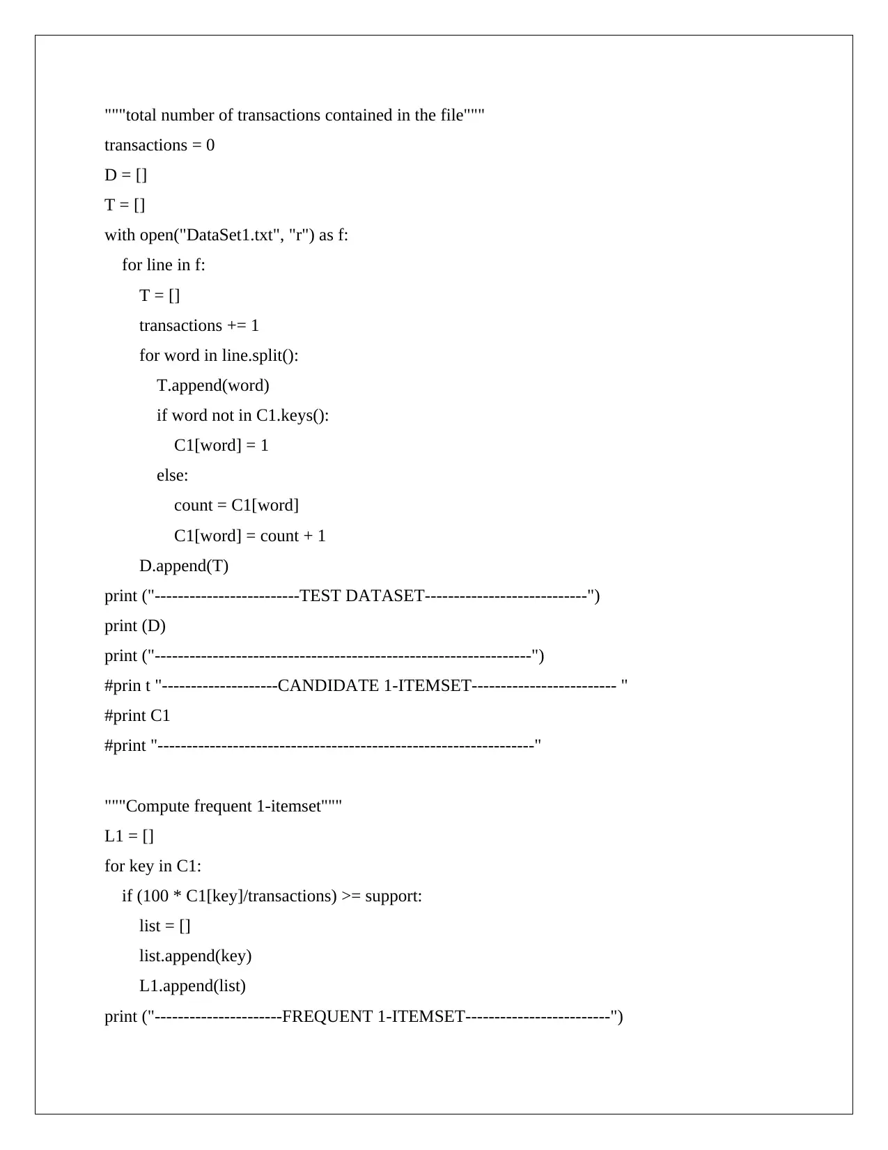
Using Python
import itertools
"""prompt user to enter support and confidence values in percent"""
support = int(input("Please enter support value in %: "))
confidence = int(input("Please enter confidence value in %: "))
"""Compute candidate 1-itemset"""
C1 = {}

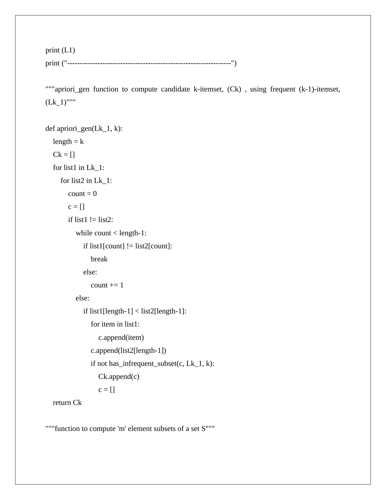
"""total number of transactions contained in the file"""
transactions = 0
D = []
T = []
with open("DataSet1.txt", "r") as f:
for line in f:
T = []
transactions += 1
for word in line.split():
T.append(word)
if word not in C1.keys():
C1[word] = 1
else:
count = C1[word]
C1[word] = count + 1
D.append(T)
print ("-------------------------TEST DATASET----------------------------")
print (D)
print ("-----------------------------------------------------------------")
#prin t "--------------------CANDIDATE 1-ITEMSET------------------------- "
#print C1
#print "-----------------------------------------------------------------"
"""Compute frequent 1-itemset"""
L1 = []
for key in C1:
if (100 * C1[key]/transactions) >= support:
list = []
list.append(key)
L1.append(list)
print ("----------------------FREQUENT 1-ITEMSET-------------------------")

print (L1)
print ("-----------------------------------------------------------------")
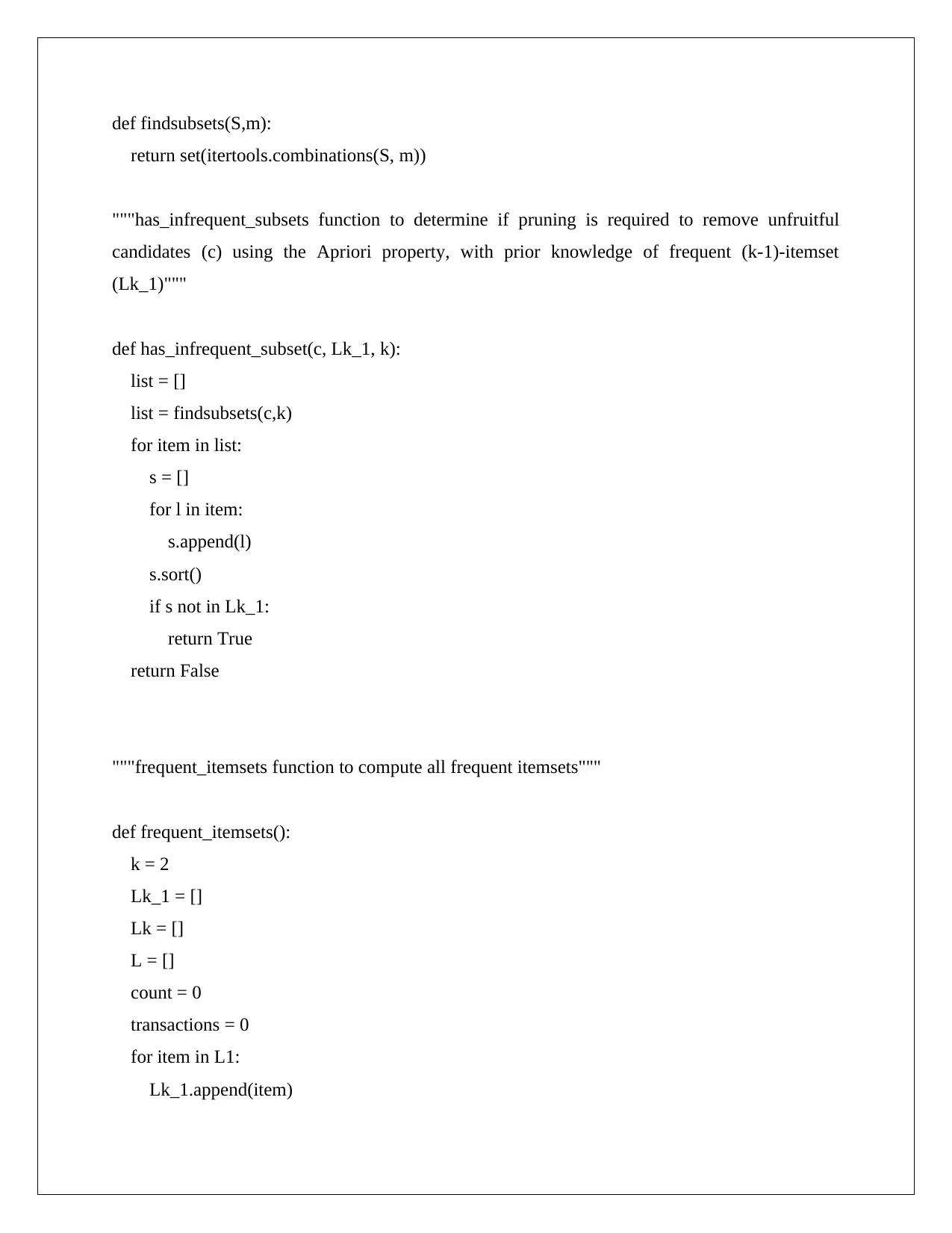
"""apriori_gen function to compute candidate k-itemset, (Ck) , using frequent (k-1)-itemset,
(Lk_1)"""
def apriori_gen(Lk_1, k):
length = k
Ck = []
for list1 in Lk_1:
for list2 in Lk_1:
count = 0
c = []
if list1 != list2:
while count < length-1:
if list1[count] != list2[count]:
break
else:
count += 1
else:
if list1[length-1] < list2[length-1]:
for item in list1:
c.append(item)
c.append(list2[length-1])
if not has_infrequent_subset(c, Lk_1, k):
Ck.append(c)
c = []
return Ck
"""function to compute 'm' element subsets of a set S"""

def findsubsets(S,m):
return set(itertools.combinations(S, m))
"""has_infrequent_subsets function to determine if pruning is required to remove unfruitful
candidates (c) using the Apriori property, with prior knowledge of frequent (k-1)-itemset
(Lk_1)"""
def has_infrequent_subset(c, Lk_1, k):
list = []
list = findsubsets(c,k)
for item in list:
s = []
for l in item:
s.append(l)
s.sort()
if s not in Lk_1:
return True
return False
"""frequent_itemsets function to compute all frequent itemsets"""
def frequent_itemsets():
k = 2
Lk_1 = []
Lk = []
L = []
count = 0
transactions = 0
for item in L1:
Lk_1.append(item)

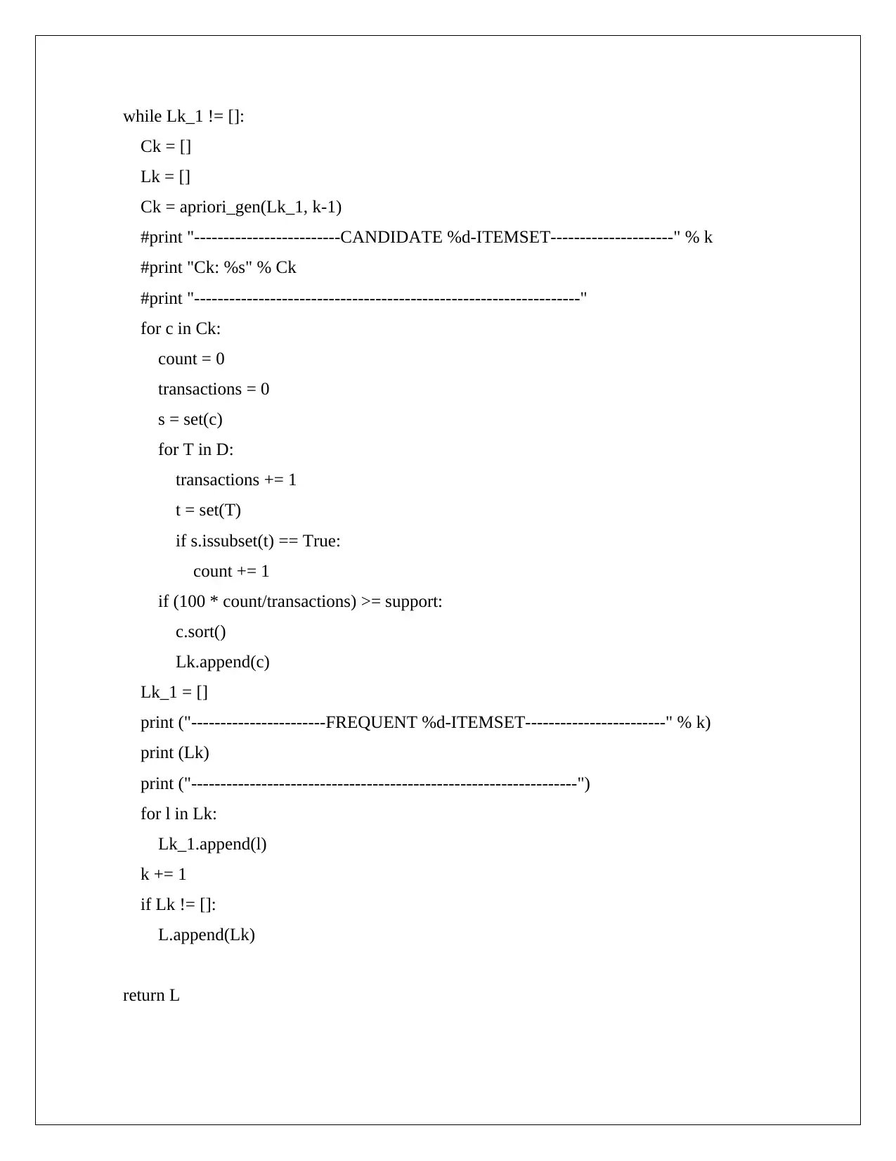
while Lk_1 != []:
Ck = []
Lk = []
Ck = apriori_gen(Lk_1, k-1)
#print "-------------------------CANDIDATE %d-ITEMSET---------------------" % k
#print "Ck: %s" % Ck
#print "------------------------------------------------------------------"
for c in Ck:
count = 0
transactions = 0
s = set(c)
for T in D:
transactions += 1
t = set(T)
if s.issubset(t) == True:
count += 1
if (100 * count/transactions) >= support:
c.sort()
Lk.append(c)
Lk_1 = []
print ("-----------------------FREQUENT %d-ITEMSET------------------------" % k)
print (Lk)
print ("------------------------------------------------------------------")
for l in Lk:
Lk_1.append(l)
k += 1
if Lk != []:
L.append(Lk)
return L

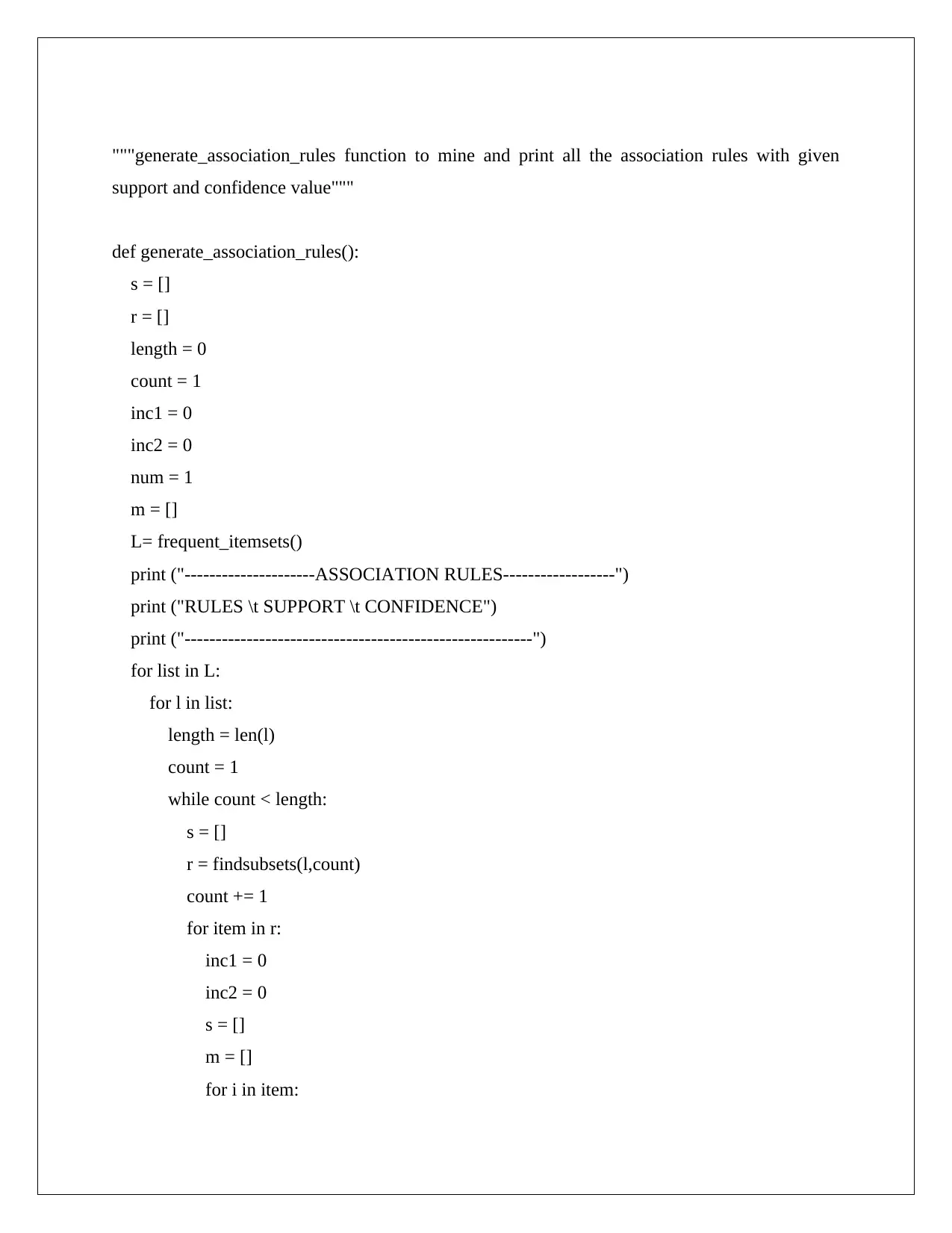
"""generate_association_rules function to mine and print all the association rules with given
support and confidence value"""
def generate_association_rules():
s = []
r = []
length = 0
count = 1
inc1 = 0
inc2 = 0
num = 1
m = []
L= frequent_itemsets()
print ("---------------------ASSOCIATION RULES------------------")
print ("RULES \t SUPPORT \t CONFIDENCE")
print ("--------------------------------------------------------")
for list in L:
for l in list:
length = len(l)
count = 1
while count < length:
s = []
r = findsubsets(l,count)
count += 1
for item in r:
inc1 = 0
inc2 = 0
s = []
m = []
for i in item:

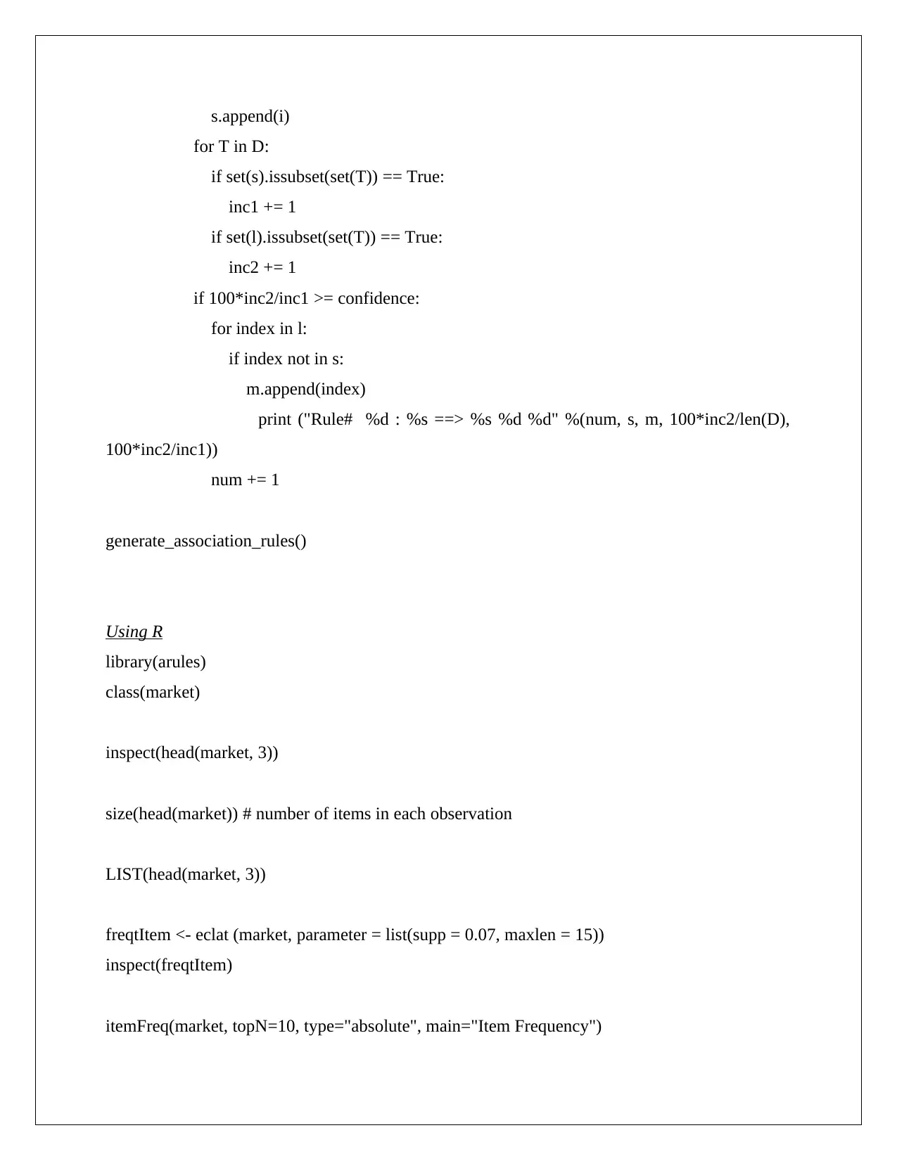
s.append(i)
for T in D:
if set(s).issubset(set(T)) == True:
inc1 += 1
if set(l).issubset(set(T)) == True:
inc2 += 1
if 100*inc2/inc1 >= confidence:
for index in l:
if index not in s:
m.append(index)
print ("Rule# %d : %s ==> %s %d %d" %(num, s, m, 100*inc2/len(D),
100*inc2/inc1))
num += 1
generate_association_rules()
Using R
library(arules)
class(market)
inspect(head(market, 3))
size(head(market)) # number of items in each observation
LIST(head(market, 3))
freqtItem <- eclat (market, parameter = list(supp = 0.07, maxlen = 15))
inspect(freqtItem)
itemFreq(market, topN=10, type="absolute", main="Item Frequency")

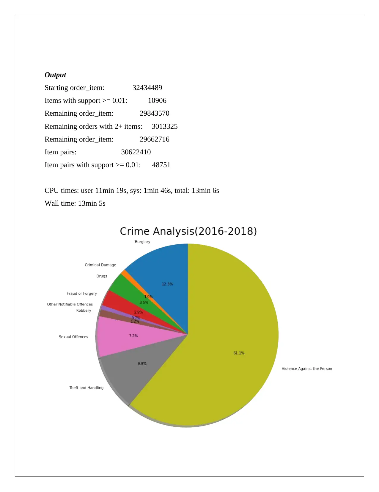
Output
Starting order_item: 32434489
Items with support >= 0.01: 10906
Remaining order_item: 29843570
Remaining orders with 2+ items: 3013325
Remaining order_item: 29662716
Item pairs: 30622410
Item pairs with support >= 0.01: 48751
CPU times: user 11min 19s, sys: 1min 46s, total: 13min 6s
Wall time: 13min 5s

Correlation
Correlation is one of the most widely used statistical concepts it providesa definitions and
intuition behind several types of correlation and illustrate how to calculate correlation using the
Python pandas library (Han et al. 2017).It is a mutually connected with association. Correlation
means one data is connected or related with another data with how much degree of similarity.
For a business purpose, It is mandatory to maintain the clarity between the pictures of customer
type and the bought items. Correlation deals with such types of topics where statistics are
essential.
Using Python
import pandas as pd
path =
mpg_data = pd.read_csv('http://archive.ics.uci.edu/ml/machine-learning-databases/auto-mpg/
auto-mpg.data', delim_whitespace=True, header=None,names = ['mpg', 'cylinder',
'displacemnt','horsepwr','weight', 'acceleration', 'model_year', 'origin', 'name'],
na_values='?')
mpg_data['mpg'].corr(mpg_data['weight'])
# pairwise correlation
mpg_data.drop(['model_year', 'origin'], axis=1).corr(method='sperman')
# plot correlated values
plt.rcParams['figure.figsize'] = [16, 6]
fig, ax = plt.subplots(nrws=1, ncls=3)
ax=ax.flatten()
cols = ['weight', 'horsepower', 'acceleration']
colors=['#415052', '#f33234', '#243AC5', '#2442B5']

j=0
for i in ax:
if j==0:
i.set_ylabel('MPG')
i.scatter(mpg_data[cols[j]], mpg_data['mpg'], alpha=0.5, color=colors[j])
i.set_xlabel(cols[j])
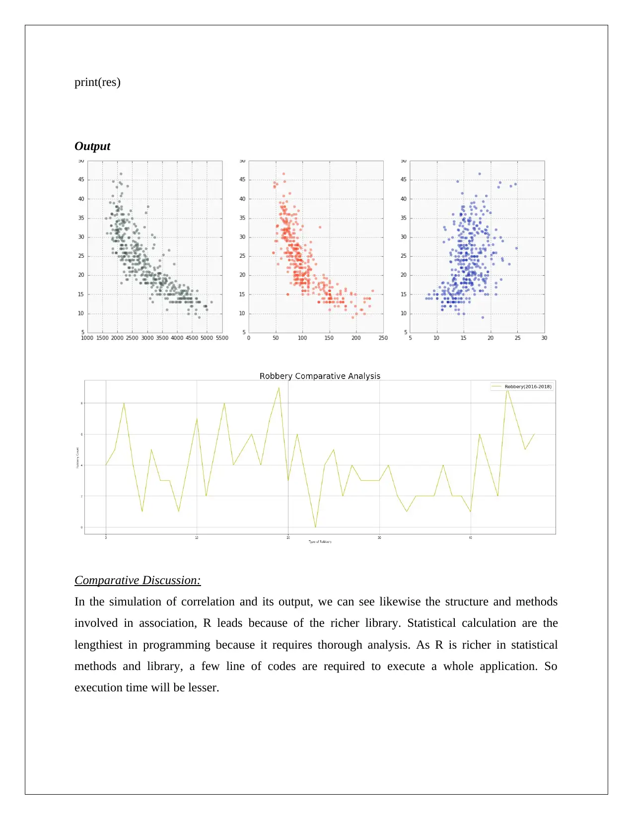
i.set_title('Pearson: %s'%mpg_data.corr().loc[cols[j]]['mpg'].round(2)+' Spearman:
%s'%mpg_data.corr(method='spearman').loc[cols[j]]['mpg'].round(2))
j+=1
plt.show()
Using R
my_data <- read.csv(file.choose())
my_data <- mtcars
head(my_data, 6)
library("ggpubr")
ggscatter(my_data, x = "mpg", y = "wt",
add = "reg.line", conf.int = TRUE,
cor.coef = TRUE, cor.method = "pearson",
xlab = "Miles/(US) gallon", ylab = "Weight (1000 lbs)")
library("ggpubr")
ggqqplot(my_data$mpg, ylab = "MPG")
ggqqplot(my_data$wt, ylab = "WT")
res <- cor.test(my_data$wt, my_data$mpg,
method = "pearson")

print(res)
Output
Comparative Discussion:
In the simulation of correlation and its output, we can see likewise the structure and methods
involved in association, R leads because of the richer library. Statistical calculation are the
lengthiest in programming because it requires thorough analysis. As R is richer in statistical
methods and library, a few line of codes are required to execute a whole application. So
execution time will be lesser.

Regression
It is the technique or algorithm to relate the input with target data set. Here the example is shown
regarding linear model. Let we see the example.
Using Python
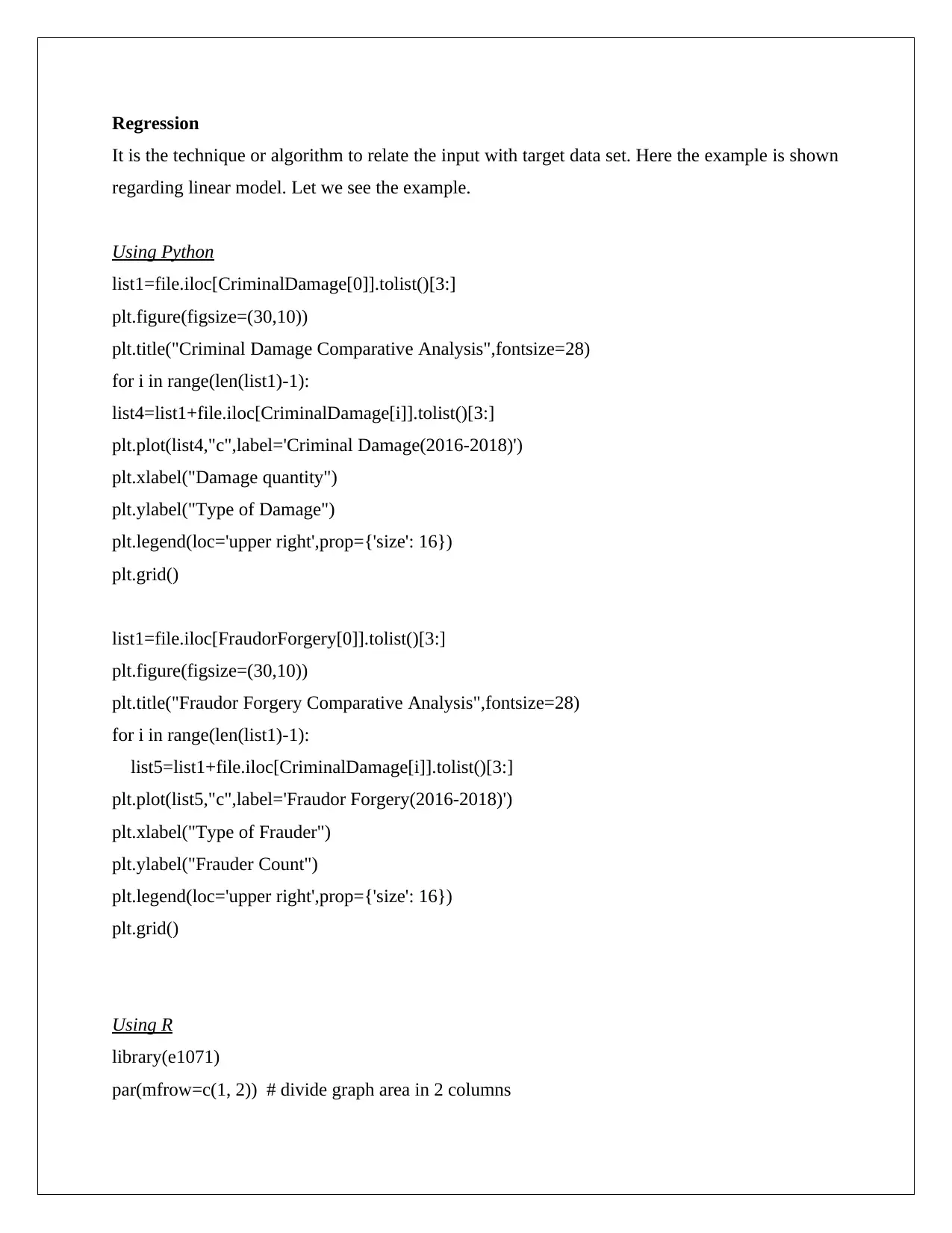
list1=file.iloc[CriminalDamage[0]].tolist()[3:]
plt.figure(figsize=(30,10))
plt.title("Criminal Damage Comparative Analysis",fontsize=28)
for i in range(len(list1)-1):
list4=list1+file.iloc[CriminalDamage[i]].tolist()[3:]
plt.plot(list4,"c",label='Criminal Damage(2016-2018)')
plt.xlabel("Damage quantity")
plt.ylabel("Type of Damage")
plt.legend(loc='upper right',prop={'size': 16})
plt.grid()
list1=file.iloc[FraudorForgery[0]].tolist()[3:]
plt.figure(figsize=(30,10))
plt.title("Fraudor Forgery Comparative Analysis",fontsize=28)
for i in range(len(list1)-1):
list5=list1+file.iloc[CriminalDamage[i]].tolist()[3:]
plt.plot(list5,"c",label='Fraudor Forgery(2016-2018)')
plt.xlabel("Type of Frauder")
plt.ylabel("Frauder Count")
plt.legend(loc='upper right',prop={'size': 16})
plt.grid()
Using R
library(e1071)
par(mfrow=c(1, 2)) # divide graph area in 2 columns

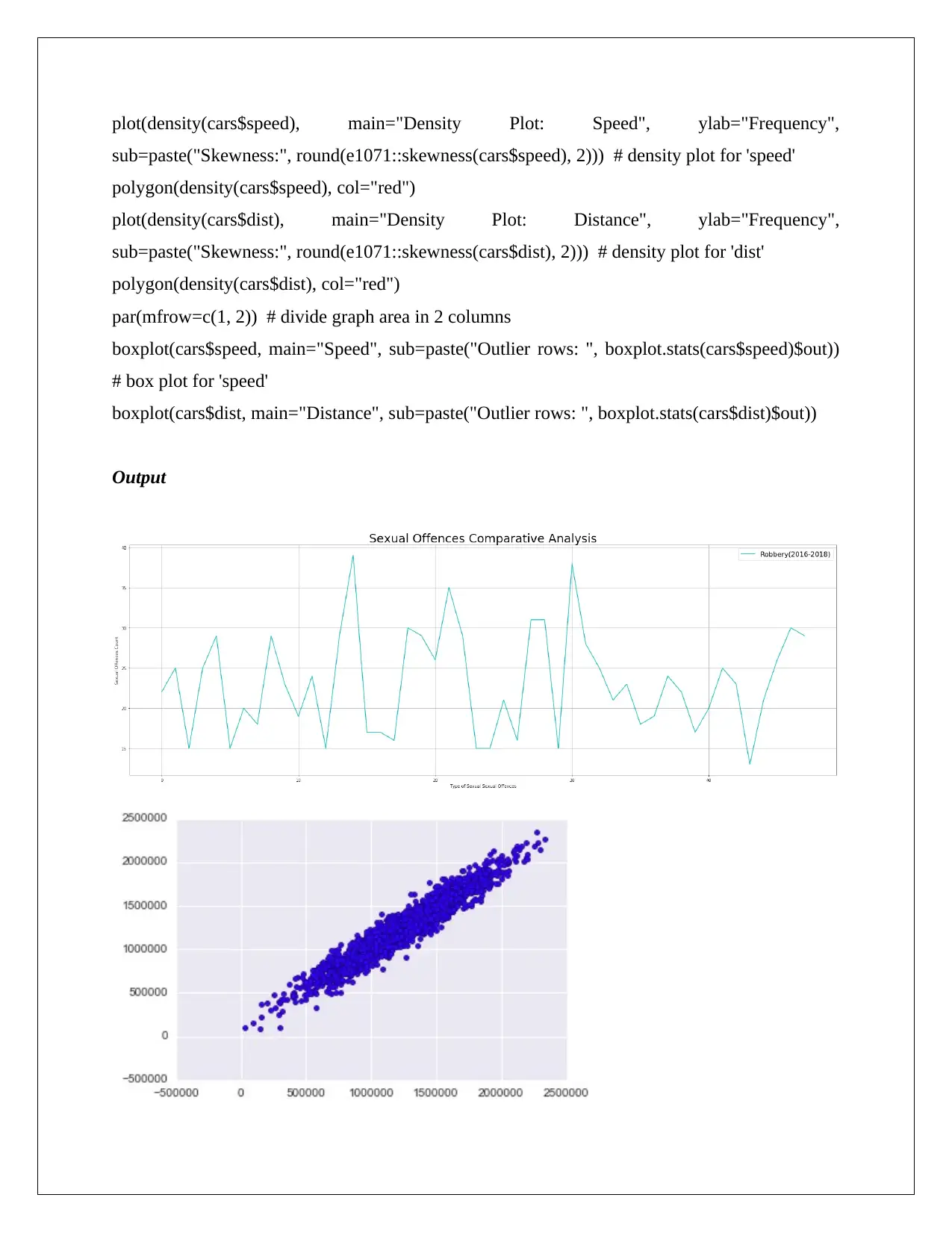
plot(density(cars$speed), main="Density Plot: Speed", ylab="Frequency",
sub=paste("Skewness:", round(e1071::skewness(cars$speed), 2))) # density plot for 'speed'
polygon(density(cars$speed), col="red")
plot(density(cars$dist), main="Density Plot: Distance", ylab="Frequency",
sub=paste("Skewness:", round(e1071::skewness(cars$dist), 2))) # density plot for 'dist'
polygon(density(cars$dist), col="red")
par(mfrow=c(1, 2)) # divide graph area in 2 columns
boxplot(cars$speed, main="Speed", sub=paste("Outlier rows: ", boxplot.stats(cars$speed)$out))
# box plot for 'speed'
boxplot(cars$dist, main="Distance", sub=paste("Outlier rows: ", boxplot.stats(cars$dist)$out))
Output

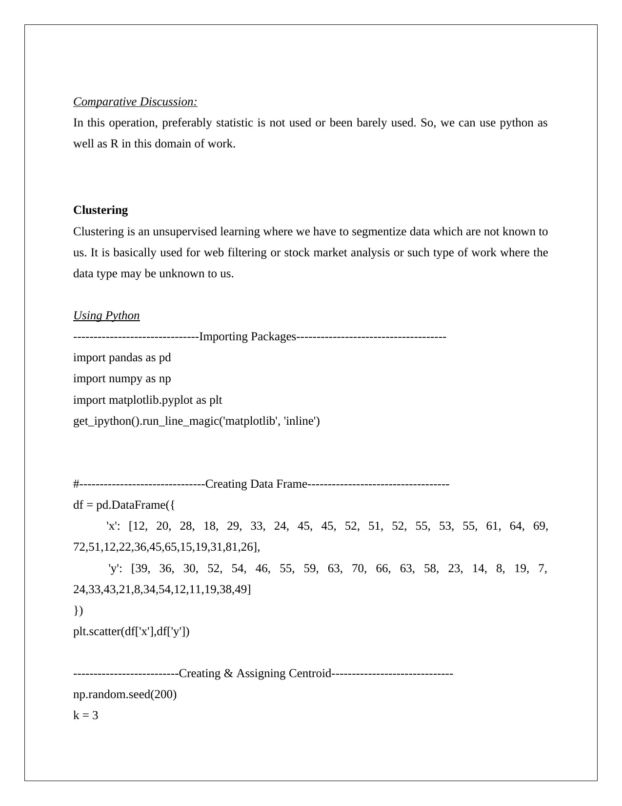
Comparative Discussion:
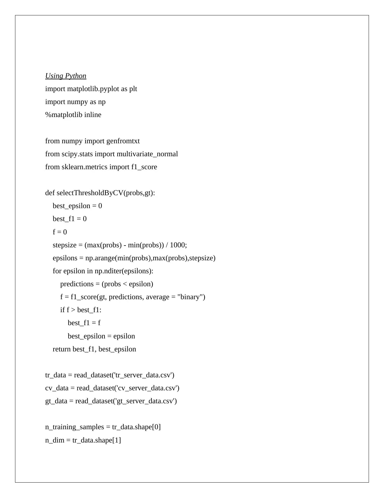
In this operation, preferably statistic is not used or been barely used. So, we can use python as
well as R in this domain of work.
Clustering
Clustering is an unsupervised learning where we have to segmentize data which are not known to
us. It is basically used for web filtering or stock market analysis or such type of work where the
data type may be unknown to us.
Using Python
-------------------------------Importing Packages-------------------------------------
import pandas as pd
import numpy as np
import matplotlib.pyplot as plt
get_ipython().run_line_magic('matplotlib', 'inline')
#-------------------------------Creating Data Frame-----------------------------------
df = pd.DataFrame({
'x': [12, 20, 28, 18, 29, 33, 24, 45, 45, 52, 51, 52, 55, 53, 55, 61, 64, 69,
72,51,12,22,36,45,65,15,19,31,81,26],
'y': [39, 36, 30, 52, 54, 46, 55, 59, 63, 70, 66, 63, 58, 23, 14, 8, 19, 7,
24,33,43,21,8,34,54,12,11,19,38,49]
})
plt.scatter(df['x'],df['y'])
--------------------------Creating & Assigning Centroid------------------------------
np.random.seed(200)
k = 3

centroids[i] = [x, y]
centroids = {
i+1: [np.random.randint(0, 80), np.random.randint(0, 80)]
for i in range(k)
}
print(centroids)
list1=[]
list1=centroids[1]
list2=centroids[2]
list3=centroids[3]
plt.figure()
a=list1[0]
b=list1[1]
plt.plot(a,b,'*r',0.6)
plt.figure()
a=list2[0]
b=list2[1]
plt.plot(a,b,'*m',0.6)
plt.figure()
a=list3[0]
b=list3[1]
plt.plot(a,b,'*c',0.6)
#-------------------------------Plotting of points(seed)-----------------------------
fig = plt.figure(figsize=(5, 5))
plt.scatter(df['x'], df['y'], color='k')
colmap = {1: 'r', 2: 'g', 3: 'b'}
for i in centroids.keys():
plt.scatter(*centroids[i], color=colmap[i])
plt.xlim(0, 80)
plt.ylim(0, 80)

plt.show()
#------------------------------ Centroid Assignment Stage(Euclidian Distance)
---------------------------
def assignment(df, centroids):
for i in centroids.keys():
# sqrt((x1 - x2)^2 - (y1 - y2)^2)
df['distance_from_{}'.format(i)] = (
np.sqrt(
(df['x'] - centroids[i][0]) ** 2
+ (df['y'] - centroids[i][1]) ** 2
)
)
centroid_distance_cols = ['distance_from_{}'.format(i) for i in centroids.keys()]
df['closest'] = df.loc[:, centroid_distance_cols].idxmin(axis=1)
df['closest'] = df['closest'].map(lambda x: int(x.lstrip('distance_from_')))
df['color'] = df['closest'].map(lambda x: colmap[x])
return df
df = assignment(df, centroids)
print(df.head(40))
#---------------------------------Plotting Seeds with Centroid-------------------------
fig = plt.figure(figsize=(5, 5))
plt.scatter(df['x'], df['y'], color=df['color'], alpha=0.5, edgecolor='k')
for i in centroids.keys():
plt.scatter(*centroids[i], color=colmap[i])
plt.xlim(0, 80)
plt.ylim(0, 80)

plt.show()
#----------------------------------------Update Stage ---------------------------------
import copy
old_centroids = copy.deepcopy(centroids)
def update(k):
for i in centroids.keys():
centroids[i][0] = np.mean(df[df['closest'] == i]['x'])
centroids[i][1] = np.mean(df[df['closest'] == i]['y'])
return k
centroids = update(centroids)
#--------------------------------Plot updated seeds in cluster form--------------------
fig = plt.figure(figsize=(5, 5))
ax = plt.axes()
plt.scatter(df['x'], df['y'], color=df['color'], alpha=0.5, edgecolor='k')
for i in centroids.keys():
plt.scatter(*centroids[i], color=colmap[i])
plt.xlim(0, 80)
plt.ylim(0, 80)
for i in old_centroids.keys():
old_x = old_centroids[i][0]
old_y = old_centroids[i][1]
dx = (centroids[i][0] - old_centroids[i][0]) * 0.75
dy = (centroids[i][1] - old_centroids[i][1]) * 0.75
ax.arrow(old_x, old_y, dx, dy, head_width=2, head_length=3, fc=colmap[i], ec=colmap[i])
plt.show()

Using R
library(VIM)
aggr(data14)
library(lubridate)
data14$Date.Time <- mdy_hms(data14$Date.Time)
data14$Year <- factor(year(data14$Date.Time))
data14$Month <- factor(month(data14$Date.Time))
data14$Day <- factor(day(data14$Date.Time))
data14$Weekday <- factor(wday(data14$Date.Time))
data14$Hour <- factor(hour(data14$Date.Time))
data14$Minute <- factor(minute(data14$Date.Time))
data14$Second <- factor(second(data14$Date.Time))
set.seed(10)
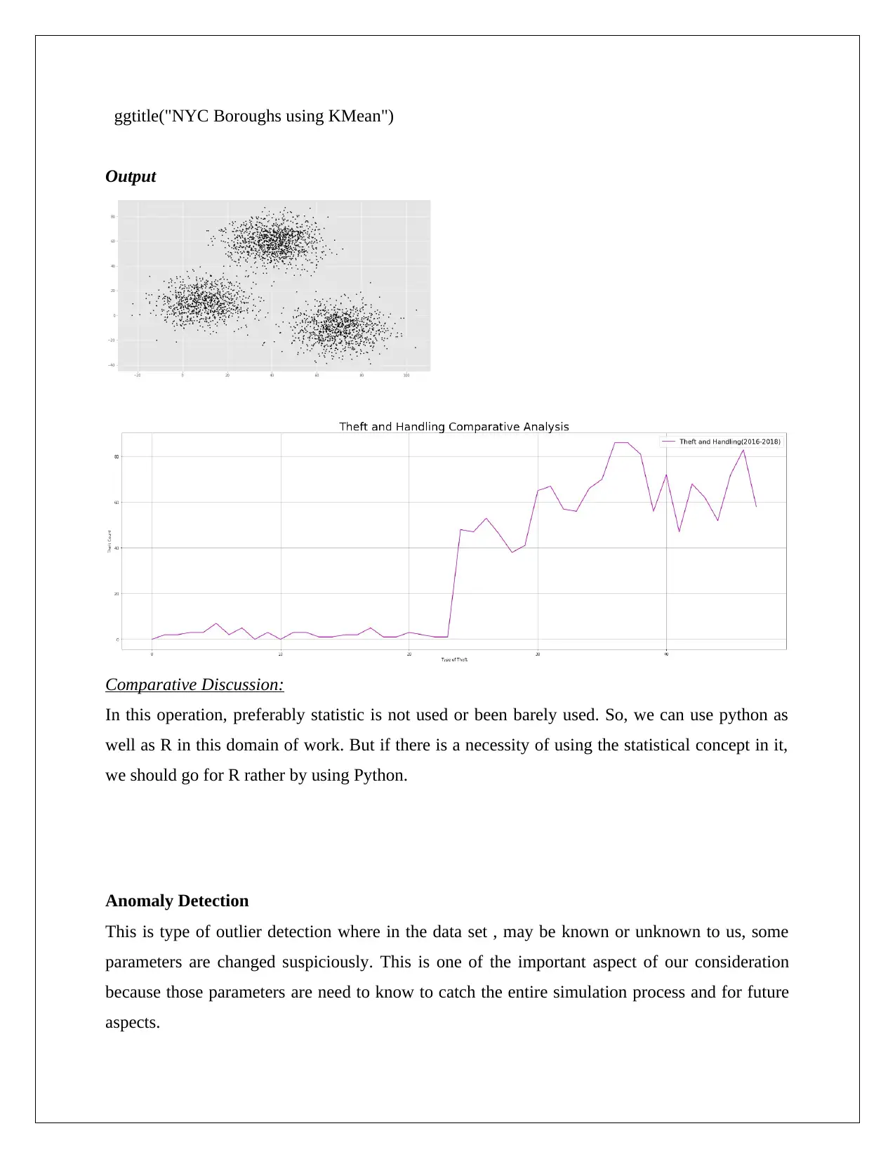
clusters <- kmeans(data14[,2:3], 5)
data14$Borough <- as.factor(clusters$cluster)
str(clusters)
library(ggmap)
NYCMap <- get_map("New York", zoom = 10)
ggmap(NYCMap) + geom_point(aes(x = Lon[], y = Lat[], colour = as.factor(Borough)),data =
data14) +

ggtitle("NYC Boroughs using KMean")
Output
Comparative Discussion:
In this operation, preferably statistic is not used or been barely used. So, we can use python as
well as R in this domain of work. But if there is a necessity of using the statistical concept in it,
we should go for R rather by using Python.
Anomaly Detection
This is type of outlier detection where in the data set , may be known or unknown to us, some
parameters are changed suspiciously. This is one of the important aspect of our consideration
because those parameters are need to know to catch the entire simulation process and for future
aspects.

Using Python
import matplotlib.pyplot as plt
import numpy as np
%matplotlib inline
from numpy import genfromtxt
from scipy.stats import multivariate_normal
from sklearn.metrics import f1_score
def selectThresholdByCV(probs,gt):
best_epsilon = 0
best_f1 = 0
f = 0
stepsize = (max(probs) - min(probs)) / 1000;
epsilons = np.arange(min(probs),max(probs),stepsize)
for epsilon in np.nditer(epsilons):
predictions = (probs < epsilon)
f = f1_score(gt, predictions, average = "binary")
if f > best_f1:
best_f1 = f
best_epsilon = epsilon
return best_f1, best_epsilon
tr_data = read_dataset('tr_server_data.csv')
cv_data = read_dataset('cv_server_data.csv')
gt_data = read_dataset('gt_server_data.csv')
n_training_samples = tr_data.shape[0]
n_dim = tr_data.shape[1]

plt.figure()
plt.xlabel("Latency (ms)")
plt.ylabel("Throughput (mb/s)")
plt.plot(tr_data[:,0],tr_data[:,1],"bx")
plt.show()
mu, sigma = estimateGaussian(tr_data)
p = multivariateGaussian(tr_data,mu,sigma)
p_cv = multivariateGaussian(cv_data,mu,sigma)
fscore, ep = selectThresholdByCV(p_cv,gt_data)
outliers = np.asarray(np.where(p < ep))
plt.figure()
plt.xlabel("Latency (ms)")
plt.ylabel("Throughput (mb/s)")
plt.plot(tr_data[:,0],tr_data[:,1],"bx") plt.plot(tr_data[outliers,0],tr_data[outliers,1],"ro")
plt.show()
Using R
library(Rcpp)
library(wikipediatrend)
library(AnomalyDetection)
fifa_data_wikipedia = wp_trend("fifa", from="2013-03-18", lang = "en")
fifa_data_wikipedia
library(ggplot2)
ggplot(fifa_data_wikipedia, aes(x=date, y=views, color=views)) + geom_line()

columns_to_keep=c("date","views")
fifa_data_wikipedia=fifa_data_wikipedia[,columns_to_keep]
anomalies = AnomalyDetectionTs(fifa_data_wikipedia, direction="pos", plot=TRUE)
anomalies$plot
anomalies$anoms
install.packages('anomalize')
library(devtools)
install_github("business-science/anomalize")
library(anomalize)
bitcoin data
library(tidyverse)
library(coindeskr)
bitcoin_data = get_historic_price(start = "2017-01-01")
bitcoin_data_ts = bitcoin_data %>% rownames_to_column() %>% as.tibble() %>% mutate(date
= as.Date(rowname)) %>% select(-one_of('rowname'))
bitcoin_data_ts %>% time_decompose(Price, method = "stl", frequency = "auto", trend = "auto")
%>% anomalize(remainder, method = "gesd", alpha = 0.05, max_anoms = 0.1) %>%
plot_anomaly_decomposition()
bitcoin_data_ts %>% time_decompose(Price) %>% anomalize(remainder) %>%
time_recompose() %>% plot_anomalies(time_recomposed = TRUE, ncol = 3, alpha_dots = 0.5)
anomalies=bitcoin_data_ts %>% time_decompose(Price)

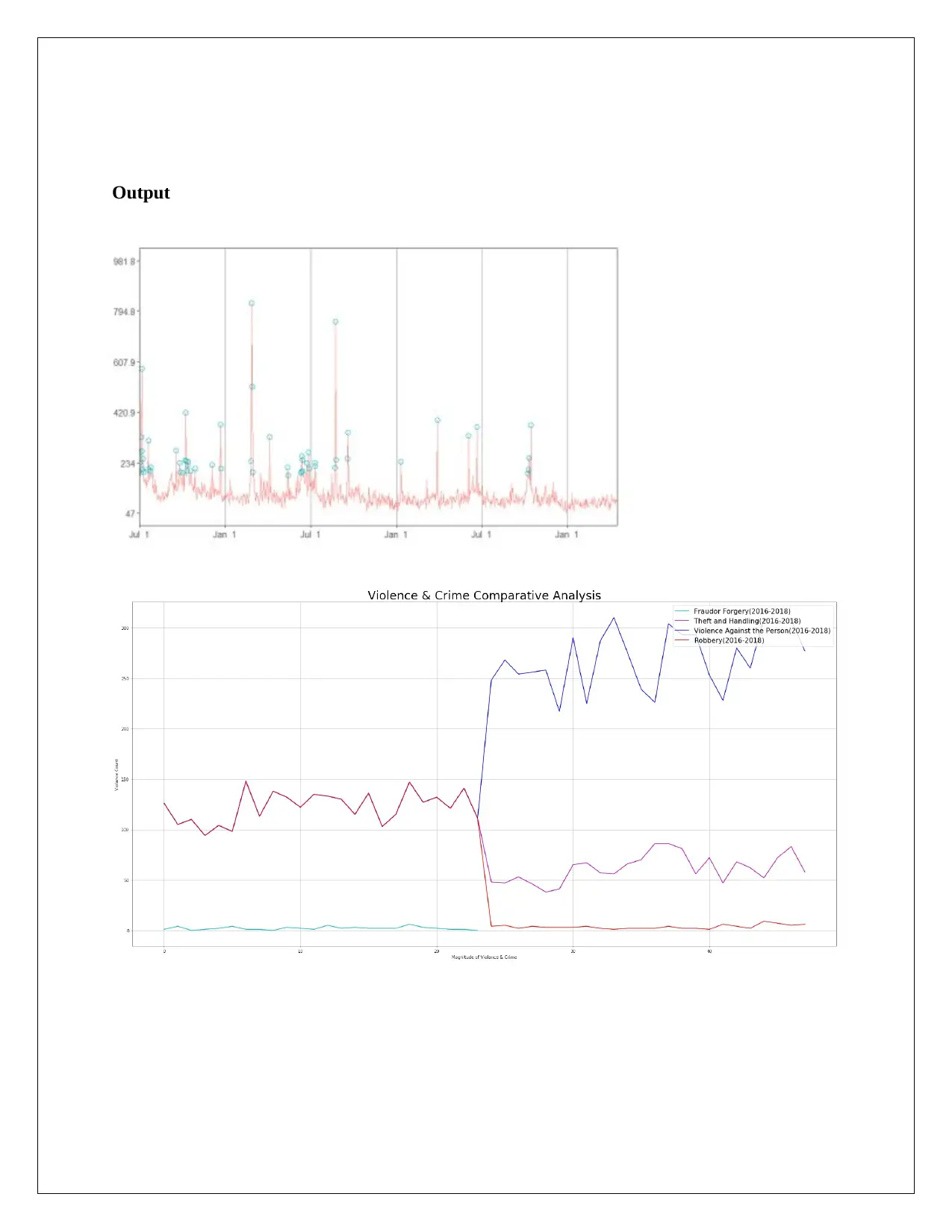
Output

Comparative Discussion:
In anomaly detection, statistical analysis is essentially required. In the example program the
simulation of bitcoin is specie which one of the most hot topic on which we can concentrate
because there are many parameters available for which the demand of bitcoin goes ups and
down.

Reference list
Gruden, G., Giunti, S., Barutta, F., Chaturvedi, N., Witte, D.R., Tricarico, M., Fuller, J.H., Perin,
P.C. and Bruno, G., 2012. QTc interval prolongation is independently associated with severe
hypoglycemic attacks in type 1 diabetes from the EURODIAB IDDM complications
study. Diabetes care, 35(1), pp.125-127.
Hunter, J.D., 2007. Matplotlib: A 2D graphics environment. Computing in science &
engineering, 9(3), pp.90-95.
Cerňak, M., 2012. A comparison of decision tree classifiers for automatic diagnosis of speech
recognition errors. Computing and Informatics, 29(3), pp.489-501.
Längkvist, M., Karlsson, L. and Loutfi, A., 2014. A review of unsupervised feature learning and
deep learning for time-series modeling. Pattern Recognition Letters, 42, pp.11-24.
Prakash, M. and Singaravel, G., 2015. An approach for prevention of privacy breach and
information leakage in sensitive data mining. Computers & Electrical Engineering, 45, pp.134-
140.
Mohammad Saeid Mahdavinejad, Mohammadreza Rezvan, Mohammadamin Barekatain,
Peyman Adibi, Payam Barnaghi, Amit P. Sheth, "Machine learning for Internet of Things data
analysis: A survey" in Digital Communications and Networks, Elsevier, 2017.
Kwon, O. and Sim, J.M., 2013. Effects of data set features on the performances of classification
algorithms. Expert Systems with Applications, 40(5), pp.1847-1857.
Han, R., John, L.K. and Zhan, J., 2018. Benchmarking big data systems: A review. IEEE
Transactions on Services Computing, 11(3), pp.580-597.
Cramer, S., Kampouridis, M., Freitas, A.A. and Alexandridis, A.K., 2017. An extensive
evaluation of seven machine learning methods for rainfall prediction in weather
derivatives. Expert Systems with Applications, 85, pp.169-181.
David, S.K., Saeb, A.T. and Al Rubeaan, K., 2013. Comparative analysis of data mining tools
and classification techniques using weka in medical bioinformatics. Computer Engineering and
Intelligent Systems, 4(13), pp.28-38.Show Context CrossRef Google Scholar

Show Context CrossRef Google Scholar
Show Context View Article Full Text: PDF (284KB) Google Scholar
Salaken, S.M., Khosravi, A., Nguyen, T. and Nahavandi, S., 2017. Extreme learning machine
based transfer learning algorithms: A survey. Neurocomputing, 267, pp.516-524.
Christensen, T.F., Lewinsky, I., Kristensen, L.E., Randlov, J., Poulsen, J.U., Eldrup, E., Pater,
C., Hejlesen, O.K. and Struijk, J.J., 2007, September. QT Interval prolongation during rapid fall
in blood glucose in type I diabetes. In Computers in Cardiology, 2007 (pp. 345-348). IEEE.
Christensen, T.F., Tarnow, L., Randløv, J., Kristensen, L.E., Struijk, J.J., Eldrup, E. and
Hejlesen, O.K., 2010. QT interval prolongation during spontaneous episodes of hypoglycaemia
in type 1 diabetes: the impact of heart rate correction. Diabetologia, 53(9), pp.2036-2041.
Kumari, V.A. and Chitra, R., 2013. Classification of diabetes disease using support vector
machine. International Journal of Engineering Research and Applications, 3(2), pp.1797-1801.
Antony, P.J., Manujesh, P. and Jnanesh, N.A., 2016, May. Data mining and machine learning
approaches on engineering materials—a review. In Recent Trends in Electronics, Information &
Communication Technology (RTEICT), IEEE International Conference on (pp. 69-73). IEEE.
Nelson, B. and Olovsson, T., 2016, December. Security and privacy for big data: A systematic
literature review. In Big Data (Big Data), 2016 IEEE International Conference on (pp. 3693-
3702). IEEE.
Dincer, C., Akpolat, G. and Zeydan, E., 2017, May. Security issues of big data applications
served by mobile operators. In Signal Processing and Communications Applications Conference
(SIU), 2017 25th (pp. 1-4). IEEE.
Volk, M., Bosse, S. and Turowski, K., 2017, July. Providing Clarity on Big Data Technologies:
A Structured Literature Review. In Business Informatics (CBI), 2017 IEEE 19th Conference
on (Vol. 1, pp. 388-397). IEEE.
Prakash, M., Padmapriy, G. and Kumar, M.V., 2018, April. A Review on Machine Learning Big
Data using R. In 2018 Second International Conference on Inventive Communication and
Computational Technologies (ICICCT) (pp. 1873-1877). IEEE.