Advanced Applied Analytical Methods 2: Investigation Report

This report presents four investigations using advanced analytical methods. The first investigation analyzes a mass-spring system, determining the spring constant, deriving equations for oscillation, and analyzing the natural frequency and time period. The second investigation explores Newton's Law of Cooling, analyzing temperature changes over time, deriving an equation for temperature, and comparing different methods. The third investigation focuses on the toughness of stainless steel, using stress-strain data to calculate the toughness of the material. The final investigation examines quality control, testing if machine stoppages follow a Poisson distribution and determining if the data is "too good to be true". The report includes detailed calculations, graphs, and explanations of the methods used.

UNIVERSITY OF DERBY
COLLEGE OF ENGINEERING AND TECHNOLOGY
MODULE TITLE: Advanced Applied Analytical Methods 2
MODULE CODE: 5ME526
Year: - 2018-2019
Applications of Advanced Analytical Methods
Pranav D. Mirani

Assignment brief:
You must complete the following 4 investigations and select suitable techniques
to analyse the data you have been given to answer the problems posed.
Your report should clearly demonstrate how you have selected and applied
suitable advanced analytical techniques to analyse the data and how your
solutions address the initial problems. You should clearly explain your
methods, why they are suitable and what the relevance is of your outcomes.
Investigation 1: Mass-Spring System (25%)
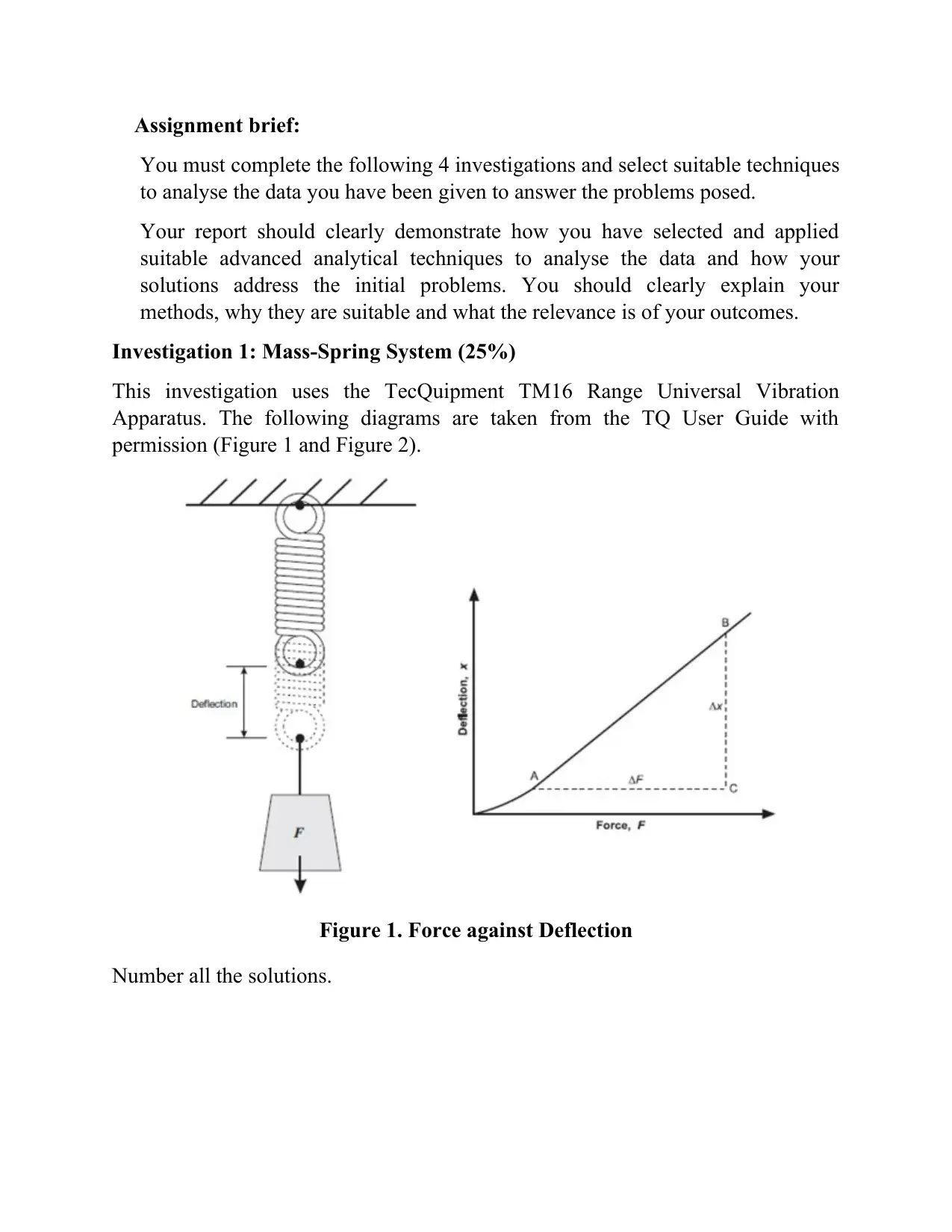
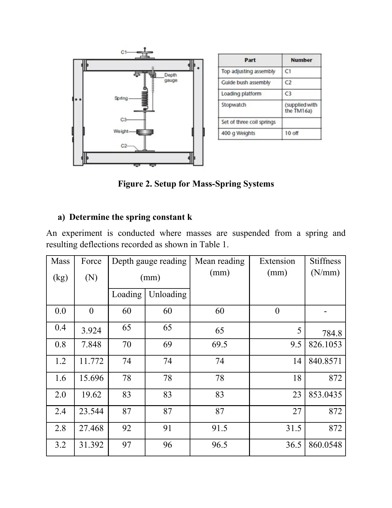
This investigation uses the TecQuipment TM16 Range Universal Vibration
Apparatus. The following diagrams are taken from the TQ User Guide with
permission (Figure 1 and Figure 2).
Figure 1. Force against Deflection
Number all the solutions.

Figure 2. Setup for Mass-Spring Systems
a) Determine the spring constant k
An experiment is conducted where masses are suspended from a spring and
resulting deflections recorded as shown in Table 1.
Mass
(kg)
Force
(N)
Depth gauge reading
(mm)
Mean reading
(mm)
Extension
(mm)
Stiffness
(N/mm)
Loading Unloading
0.0 0 60 60 60 0 -
0.4 3.924 65 65 65 5 784.8
0.8 7.848 70 69 69.5 9.5 826.1053
1.2 11.772 74 74 74 14 840.8571
1.6 15.696 78 78 78 18 872
2.0 19.62 83 83 83 23 853.0435
2.4 23.544 87 87 87 27 872
2.8 27.468 92 91 91.5 31.5 872
3.2 31.392 97 96 96.5 36.5 860.0548

3.6 35.316 101 101 101 41 861.3659
4.0 39.24 105 105 105 45 872
Coil diameter 44.6 mm
Wire diameter 3.1 mm
Number of
coils
18
Table 1. Experimentally Measured Spring Deflections for Applied Masses
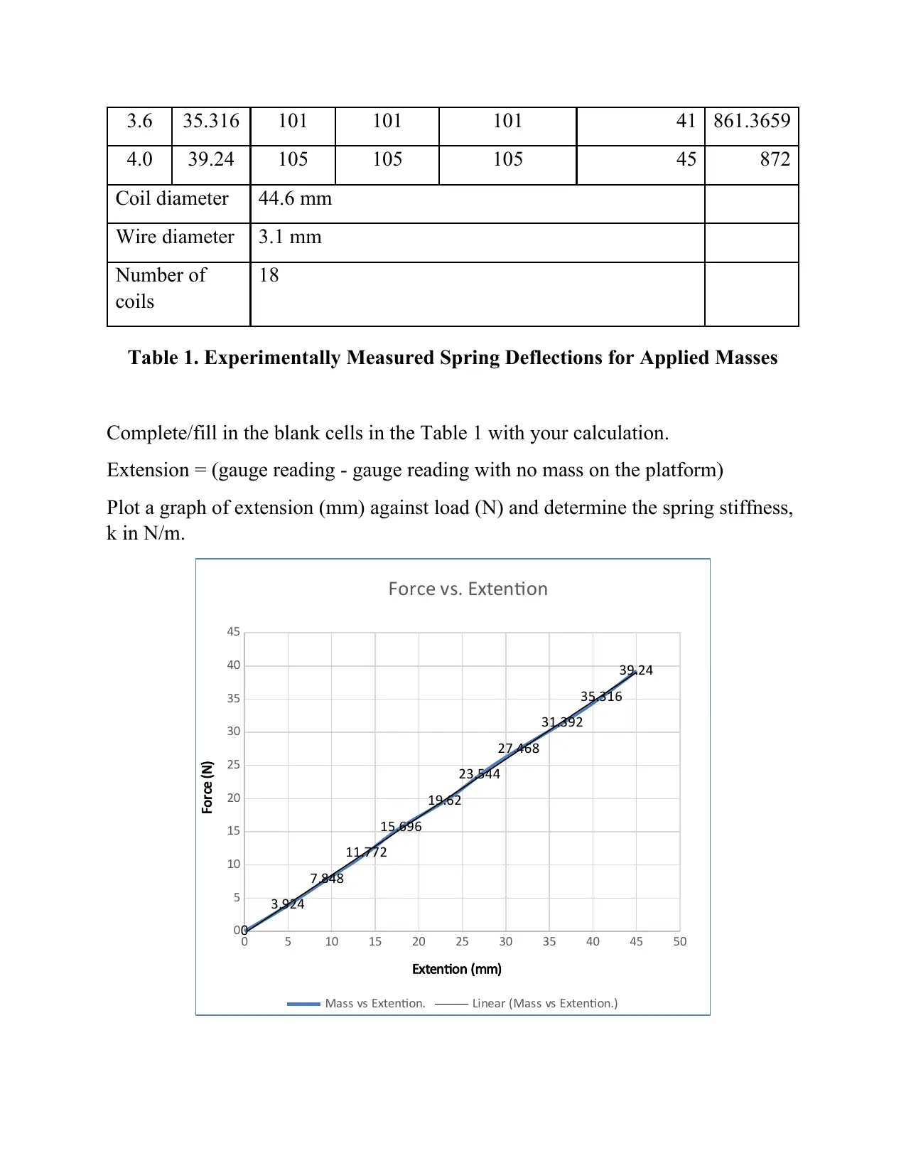
Complete/fill in the blank cells in the Table 1 with your calculation.
Extension = (gauge reading - gauge reading with no mass on the platform)
Plot a graph of extension (mm) against load (N) and determine the spring stiffness,
k in N/m.
0 5 10 15 20 25 30 35 40 45 50
0
5
10
15
20
25
30
35
40
45
0
3.924
7.848
11.772
15.696
19.62
23.544
27.468
31.392
35.316
39.24
Force vs. Extention
Mass vs Extention. Linear (Mass vs Extention.)
Extention (mm)
Force (N)

Mean stiffness of the spring = 851.4226532 N/m
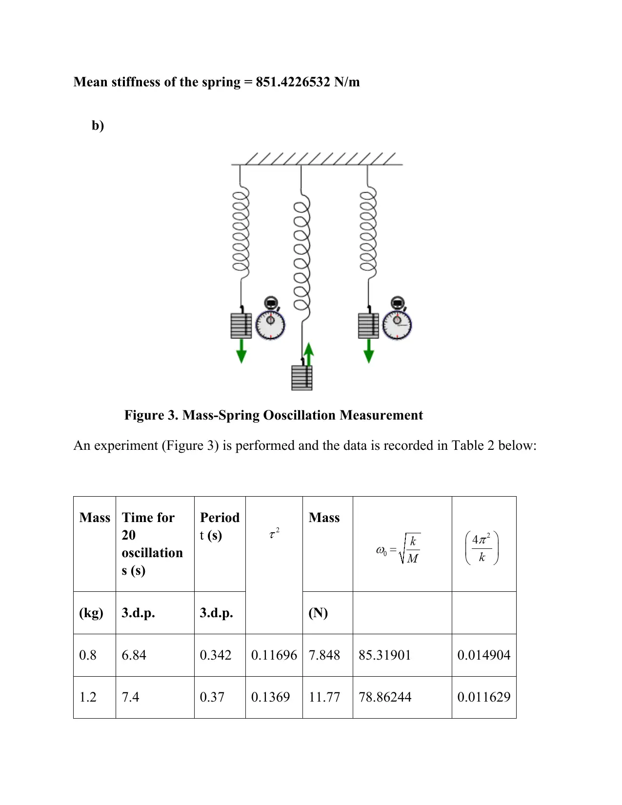
b)
Figure 3. Mass-Spring Ooscillation Measurement
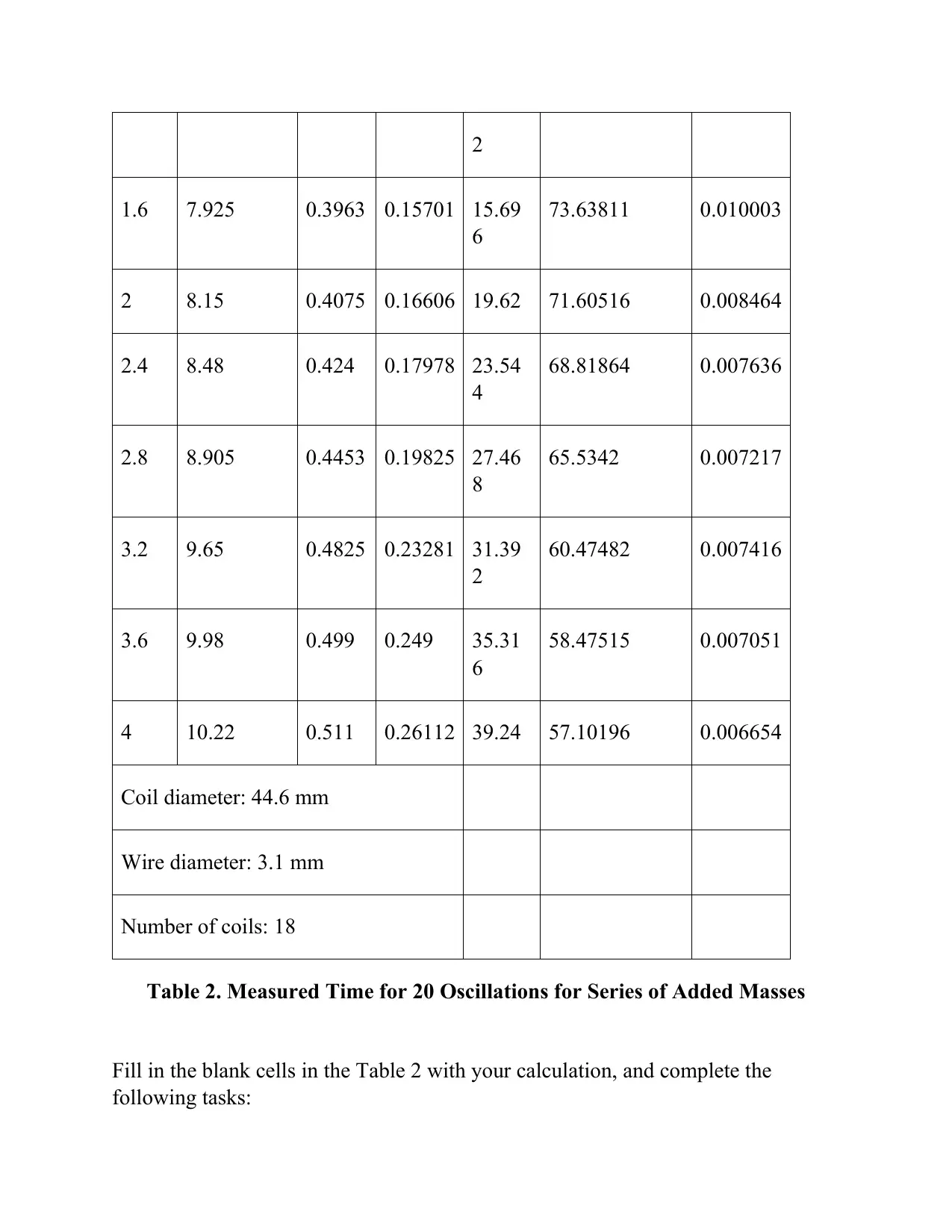
An experiment (Figure 3) is performed and the data is recorded in Table 2 below:
Mass Time for
20
oscillation
s (s)
Period
t (s)
Mass
(kg) 3.d.p. 3.d.p. (N)
0.8 6.84 0.342 0.11696 7.848 85.31901 0.014904
1.2 7.4 0.37 0.1369 11.77 78.86244 0.011629

2
1.6 7.925 0.3963 0.15701 15.69
6
73.63811 0.010003
2 8.15 0.4075 0.16606 19.62 71.60516 0.008464
2.4 8.48 0.424 0.17978 23.54
4
68.81864 0.007636
2.8 8.905 0.4453 0.19825 27.46
8
65.5342 0.007217
3.2 9.65 0.4825 0.23281 31.39
2
60.47482 0.007416
3.6 9.98 0.499 0.249 35.31
6
58.47515 0.007051
4 10.22 0.511 0.26112 39.24 57.10196 0.006654
Coil diameter: 44.6 mm
Wire diameter: 3.1 mm
Number of coils: 18
Table 2. Measured Time for 20 Oscillations for Series of Added Masses
Fill in the blank cells in the Table 2 with your calculation, and complete the
following tasks:

(i) Derive an equation from first principles to model the mass-spring
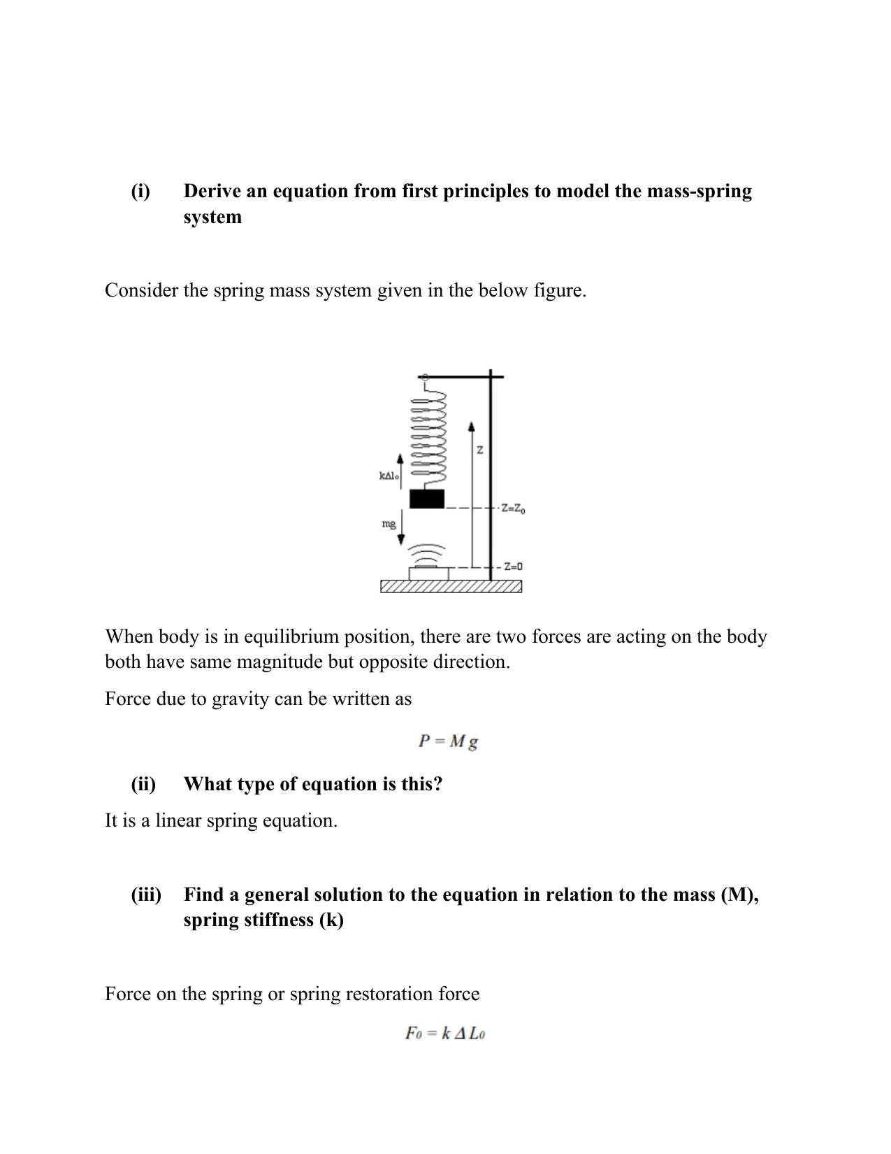
system
Consider the spring mass system given in the below figure.
When body is in equilibrium position, there are two forces are acting on the body
both have same magnitude but opposite direction.
Force due to gravity can be written as
(ii) What type of equation is this?
It is a linear spring equation.
(iii) Find a general solution to the equation in relation to the mass (M),
spring stiffness (k)
Force on the spring or spring restoration force

From the above two equations,
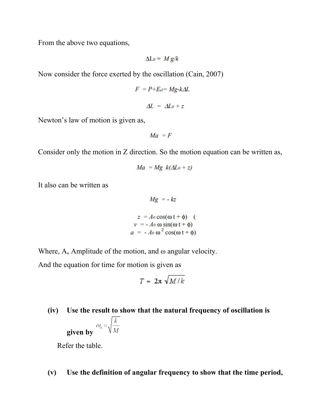
Now consider the force exerted by the oscillation (Cain, 2007)
Newton’s law of motion is given as,
Consider only the motion in Z direction. So the motion equation can be written as,
It also can be written as
Where, Ao Amplitude of the motion, and ω angular velocity.
And the equation for time for motion is given as
(iv) Use the result to show that the natural frequency of oscillation is
given by
Refer the table.
(v) Use the definition of angular frequency to show that the time period,

Refer the table.
(vi) Explain simply why the equation for is written as in part
(V)
In the equation other than M all are constant so that we written all the
constants cumulatively. During the calculation we can easily find the time by
multiplying the square root of the mass with this calculated constant value.
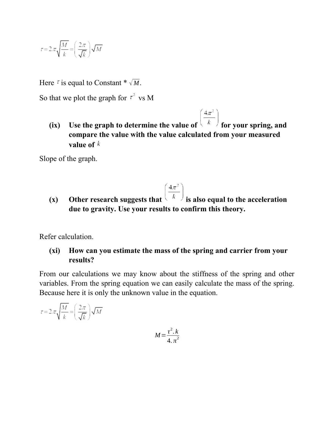
(vii) Use a spreadsheet to calculate values of and M. Plot a graph of
against M using a spreadsheet.
5 10 15 20 25 30 35 40 45
0
0.05
0.1
0.15
0.2
0.25
0.3
Mass Vs Time of Oscilation
Mass (N)
Time (Sec)
(viii) Explain why the graph of is drawn rather than the graph of
Consider the spring equation,

Here is equal to Constant * √ M.
So that we plot the graph for vs M
(ix) Use the graph to determine the value of for your spring, and
compare the value with the value calculated from your measured
value of
Slope of the graph.
(x) Other research suggests that is also equal to the acceleration
due to gravity. Use your results to confirm this theory.
Refer calculation.
(xi) How can you estimate the mass of the spring and carrier from your
results?
From our calculations we may know about the stiffness of the spring and other
variables. From the spring equation we can easily calculate the mass of the spring.
Because here it is only the unknown value in the equation.
M = τ2 . k
4. π2

Investigation 2: Newton’s Law of Cooling (25%)
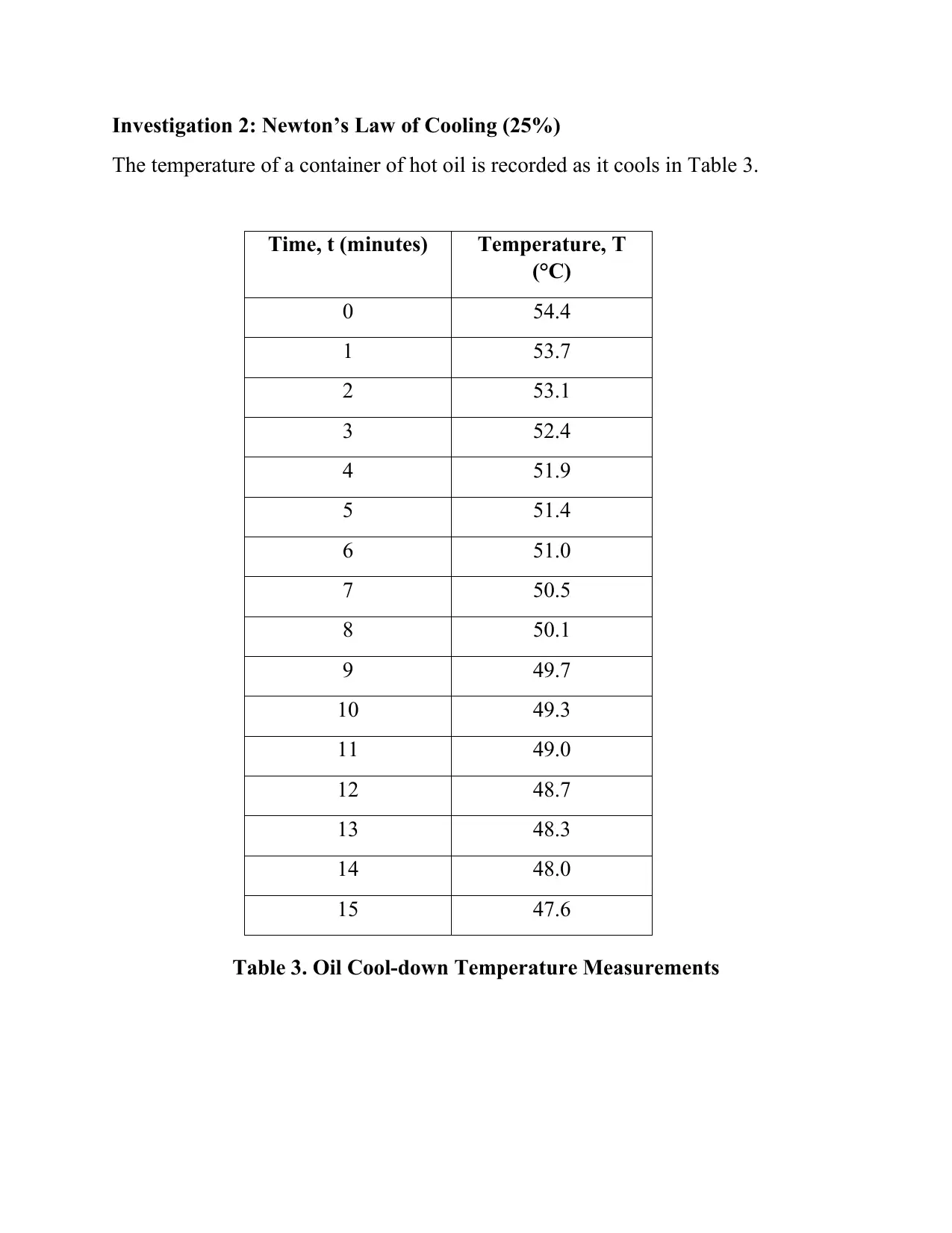
The temperature of a container of hot oil is recorded as it cools in Table 3.
Time, t (minutes) Temperature, T
(°C)
0 54.4
1 53.7
2 53.1
3 52.4
4 51.9
5 51.4
6 51.0
7 50.5
8 50.1
9 49.7
10 49.3
11 49.0
12 48.7
13 48.3
14 48.0
15 47.6
Table 3. Oil Cool-down Temperature Measurements

Complete the following tasks:
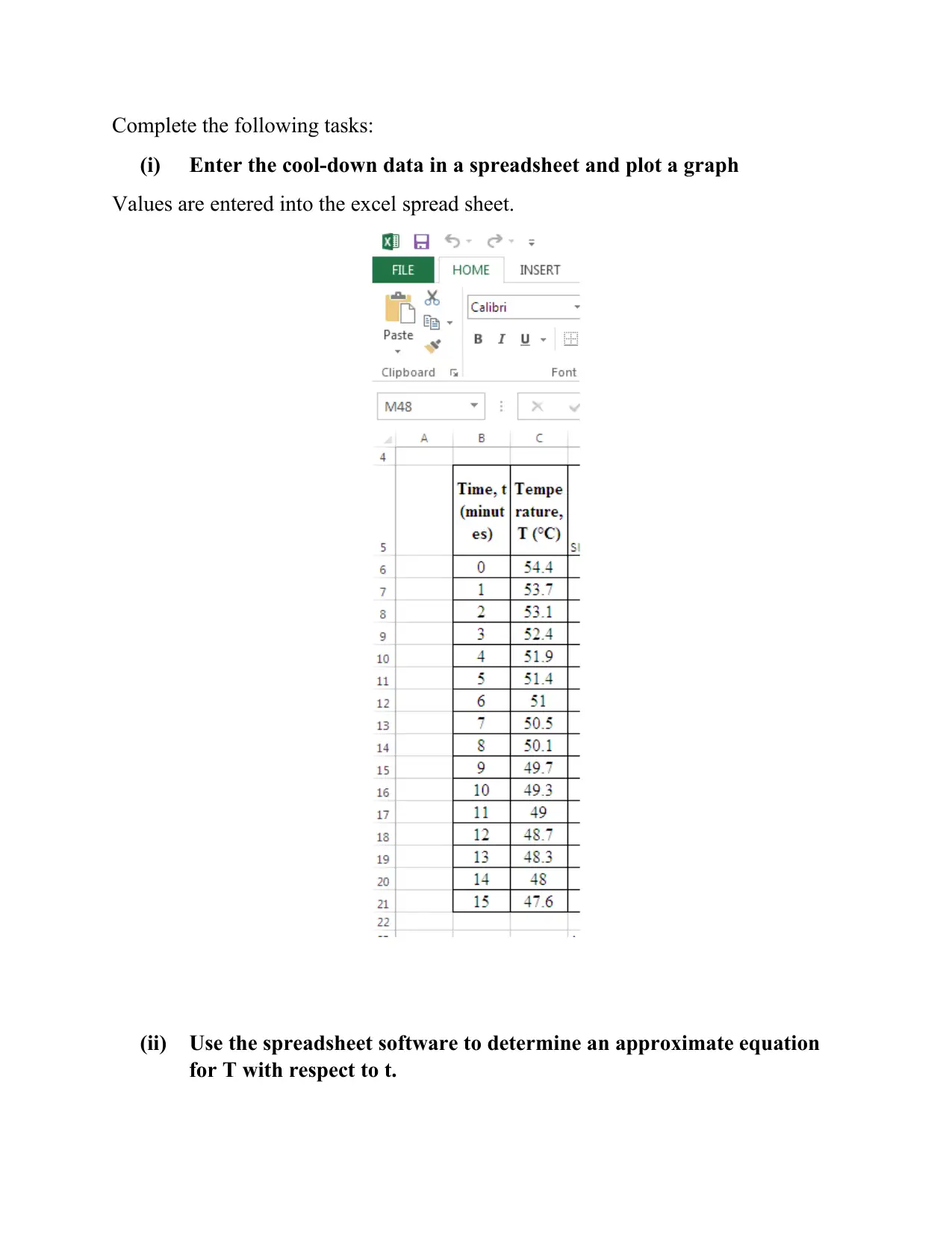
(i) Enter the cool-down data in a spreadsheet and plot a graph
Values are entered into the excel spread sheet.
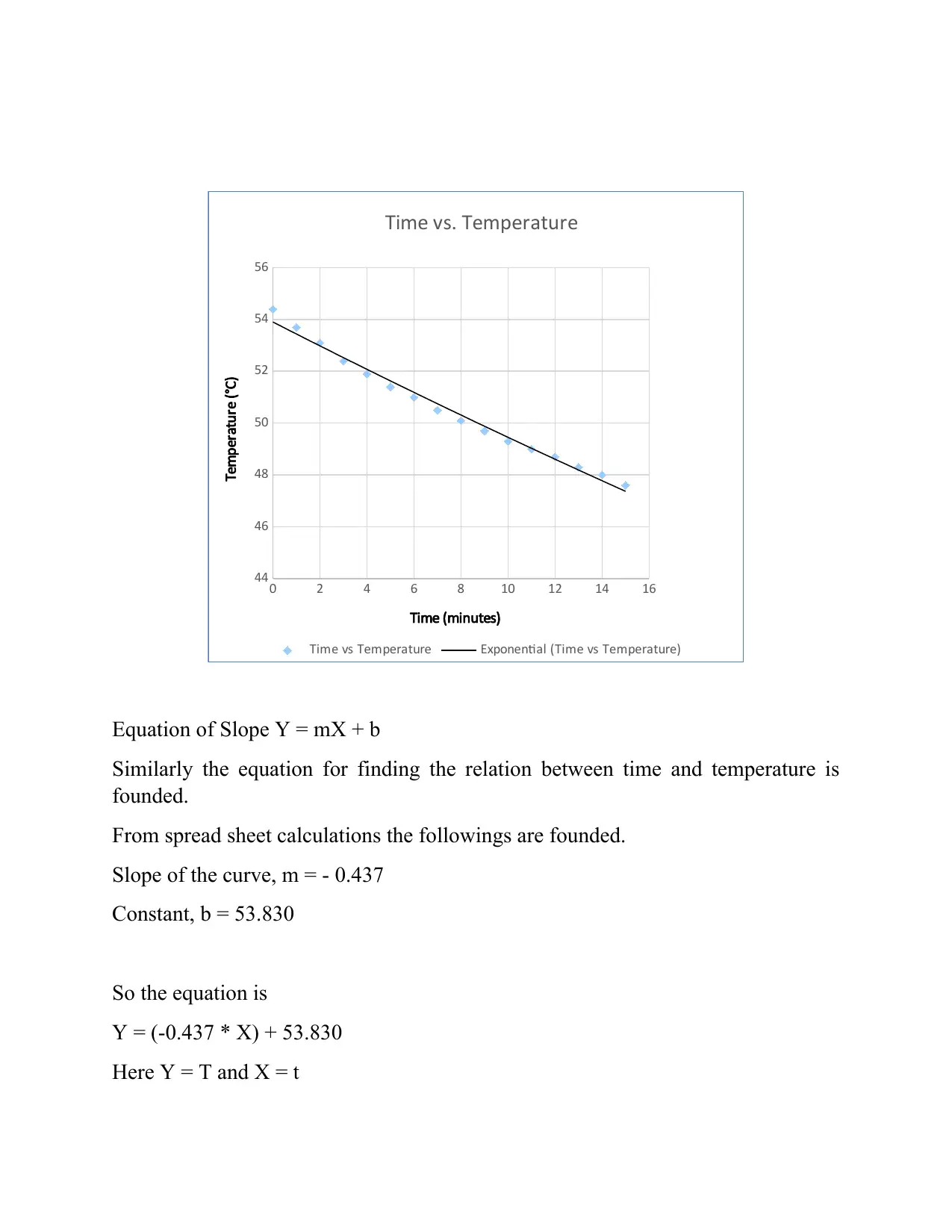
(ii) Use the spreadsheet software to determine an approximate equation
for T with respect to t.

0 2 4 6 8 10 12 14 16
44
46
48
50
52
54
56
Time vs. Temperature
Time vs Temperature Exponential (Time vs Temperature)
Time (minutes)
Temperature (°C)
Equation of Slope Y = mX + b
Similarly the equation for finding the relation between time and temperature is
founded.
From spread sheet calculations the followings are founded.
Slope of the curve, m = - 0.437
Constant, b = 53.830
So the equation is
Y = (-0.437 * X) + 53.830
Here Y = T and X = t

So the equation becomes
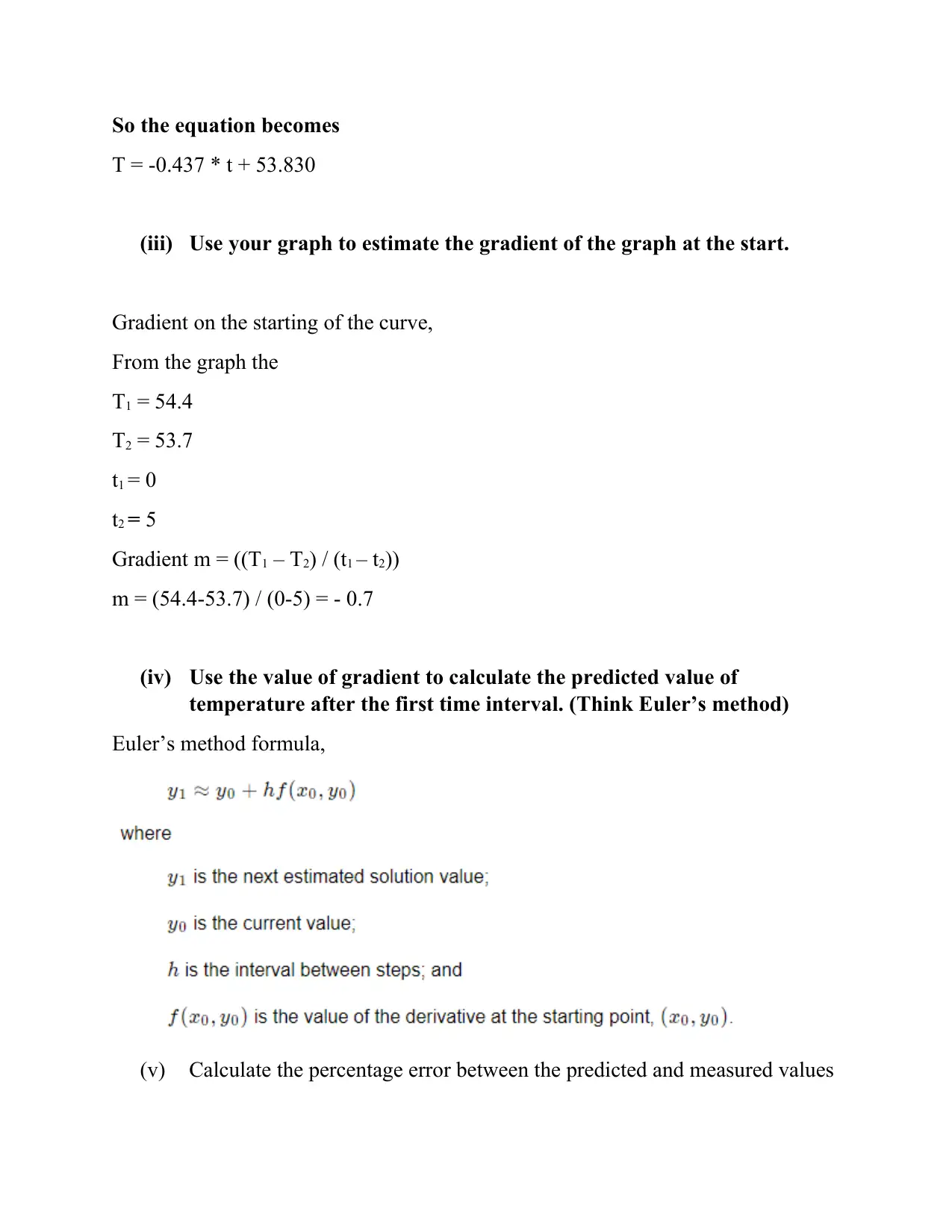
T = -0.437 * t + 53.830
(iii) Use your graph to estimate the gradient of the graph at the start.
Gradient on the starting of the curve,
From the graph the
T1 = 54.4
T2 = 53.7
t1 = 0
t2 = 5
Gradient m = ((T1 – T2) / (t1 – t2))
m = (54.4-53.7) / (0-5) = - 0.7
(iv) Use the value of gradient to calculate the predicted value of
temperature after the first time interval. (Think Euler’s method)
Euler’s method formula,
(v) Calculate the percentage error between the predicted and measured values

Calculation 1
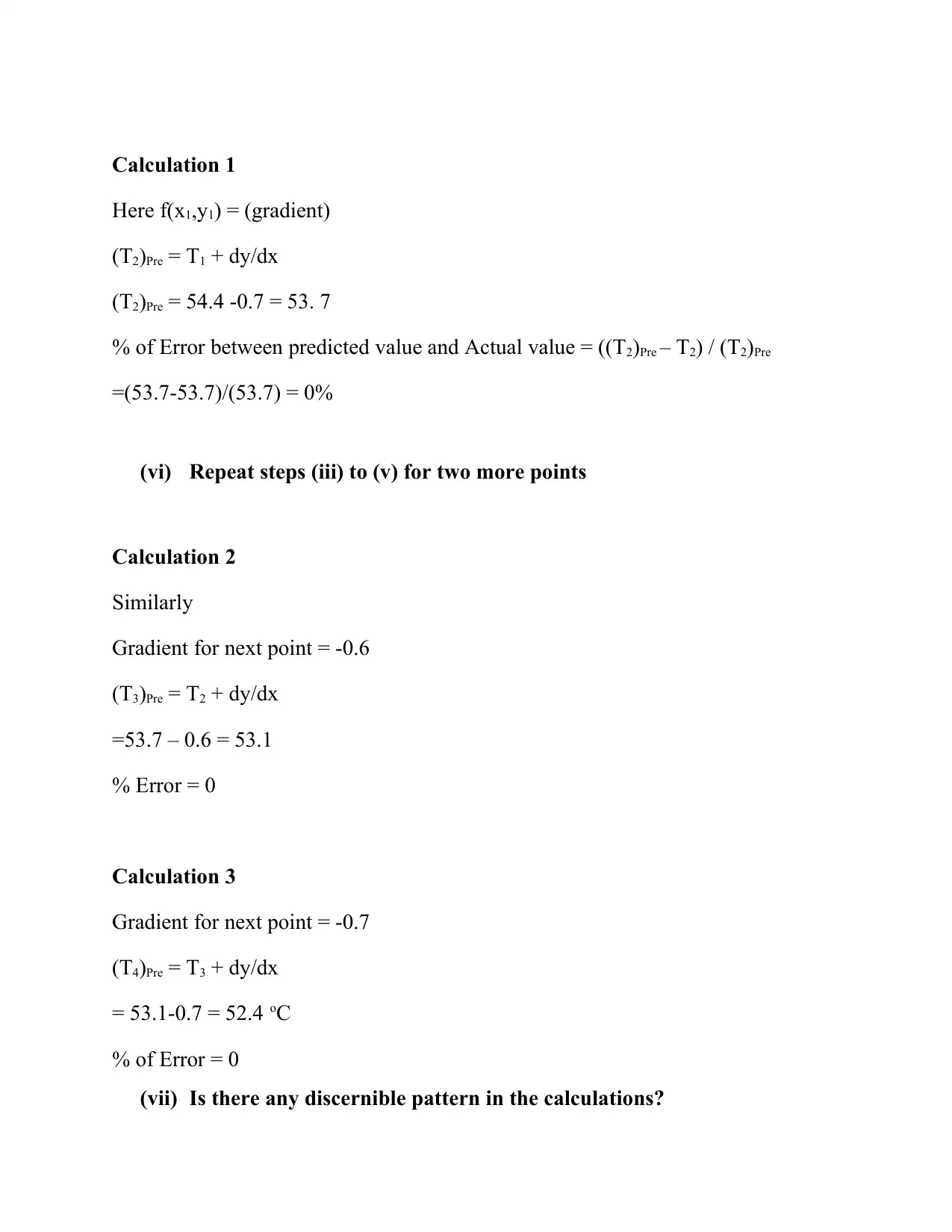
Here f(x1,y1) = (gradient)
(T2)Pre = T1 + dy/dx
(T2)Pre = 54.4 -0.7 = 53. 7
% of Error between predicted value and Actual value = ((T2)Pre – T2) / (T2)Pre
=(53.7-53.7)/(53.7) = 0%
(vi) Repeat steps (iii) to (v) for two more points
Calculation 2
Similarly
Gradient for next point = -0.6
(T3)Pre = T2 + dy/dx
=53.7 – 0.6 = 53.1
% Error = 0
Calculation 3
Gradient for next point = -0.7
(T4)Pre = T3 + dy/dx
= 53.1-0.7 = 52.4 oC
% of Error = 0
(vii) Is there any discernible pattern in the calculations?

From the above calculations that is clear the percentage of error values are zero.
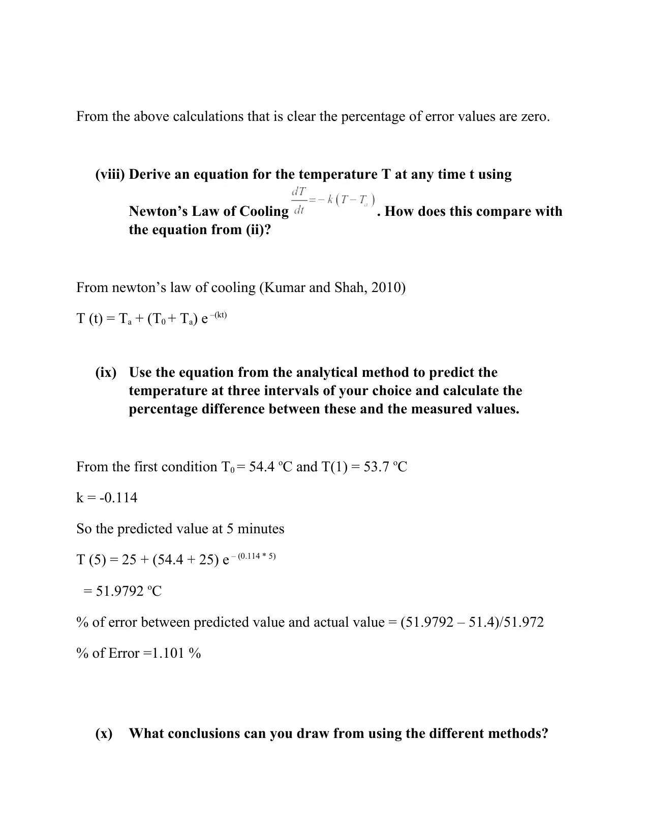
(viii) Derive an equation for the temperature T at any time t using
Newton’s Law of Cooling . How does this compare with
the equation from (ii)?
From newton’s law of cooling (Kumar and Shah, 2010)
T (t) = Ta + (T0 + Ta) e –(kt)
(ix) Use the equation from the analytical method to predict the
temperature at three intervals of your choice and calculate the
percentage difference between these and the measured values.
From the first condition T0 = 54.4 oC and T(1) = 53.7 oC
k = -0.114
So the predicted value at 5 minutes
T (5) = 25 + (54.4 + 25) e – (0.114 * 5)
= 51.9792 oC
% of error between predicted value and actual value = (51.9792 – 51.4)/51.972
% of Error =1.101 %
(x) What conclusions can you draw from using the different methods?

Here the temperature value predicted by using various methods. Among the
different methods the Euler’s method has the less error than newton’s law cooling
method.

Investigation 3: Toughness of Stainless Steel (25%)
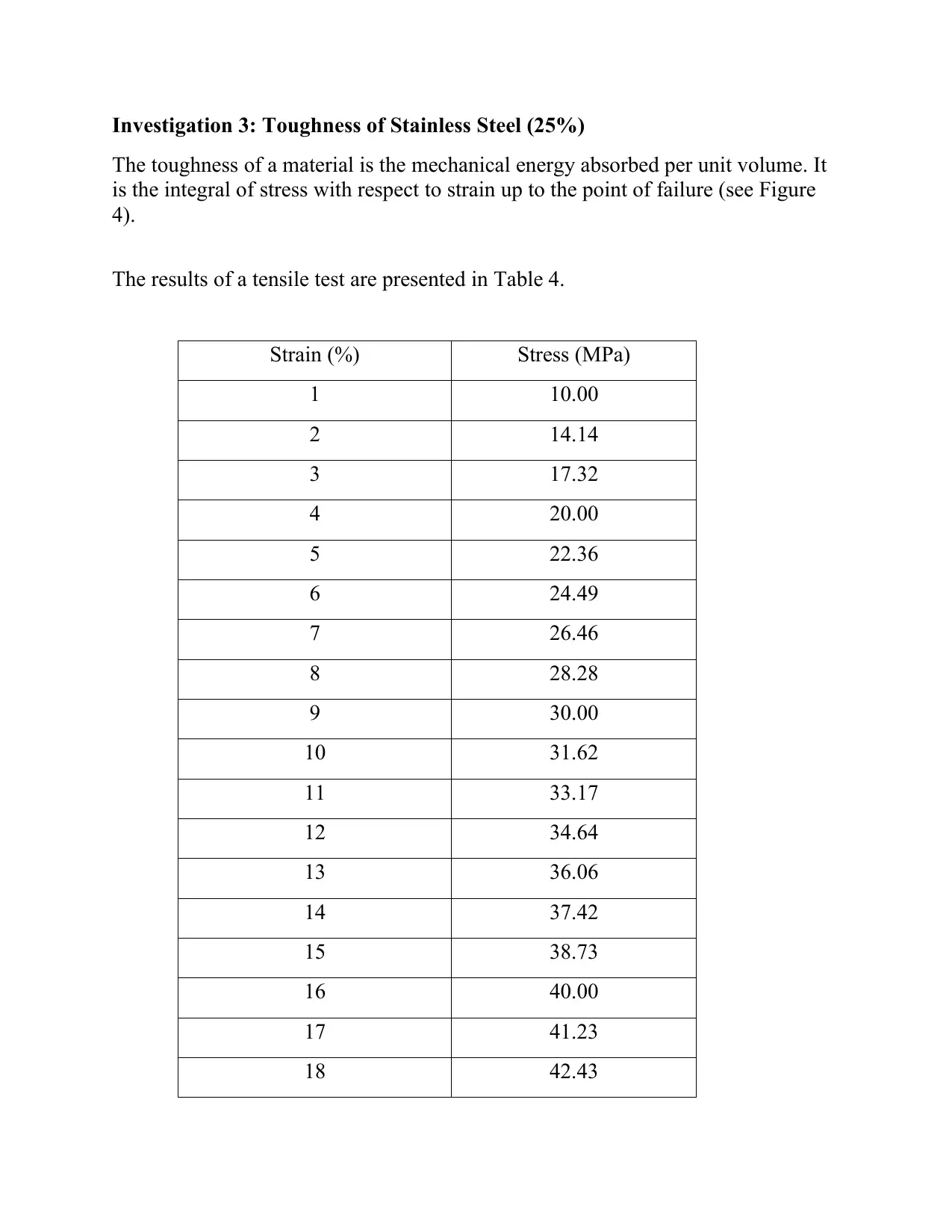
The toughness of a material is the mechanical energy absorbed per unit volume. It
is the integral of stress with respect to strain up to the point of failure (see Figure
4).
The results of a tensile test are presented in Table 4.
Strain (%) Stress (MPa)
1 10.00
2 14.14
3 17.32
4 20.00
5 22.36
6 24.49
7 26.46
8 28.28
9 30.00
10 31.62
11 33.17
12 34.64
13 36.06
14 37.42
15 38.73
16 40.00
17 41.23
18 42.43

19 43.59
20 44.72
21 45.83
22 46.90
23 47.96
24 48.99
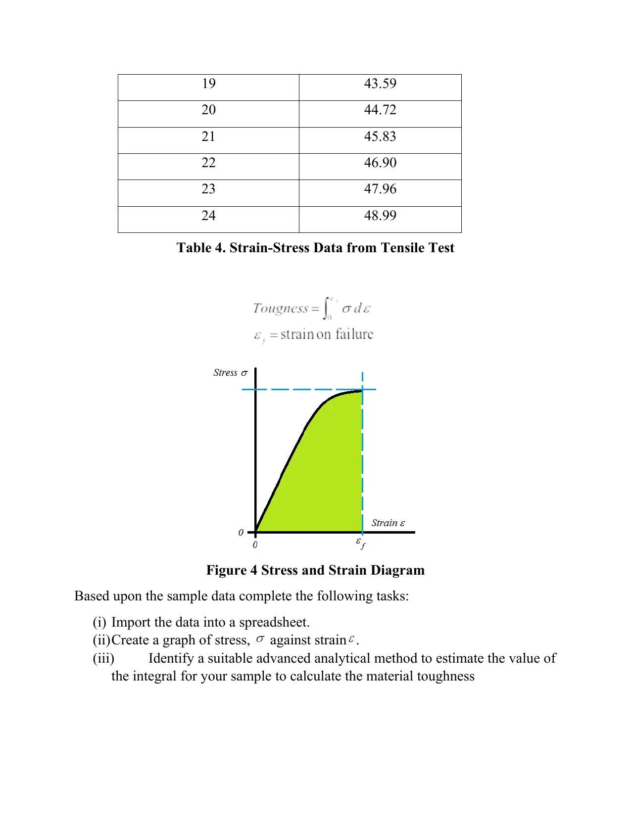
Table 4. Strain-Stress Data from Tensile Test
Figure 4 Stress and Strain Diagram
Based upon the sample data complete the following tasks:
(i) Import the data into a spreadsheet.
(ii)Create a graph of stress, against strain .
(iii) Identify a suitable advanced analytical method to estimate the value of
the integral for your sample to calculate the material toughness

0 5 10 15 20 25 30
0
10
20
30
40
50
60
Strain (%)
Stress (Mpa)
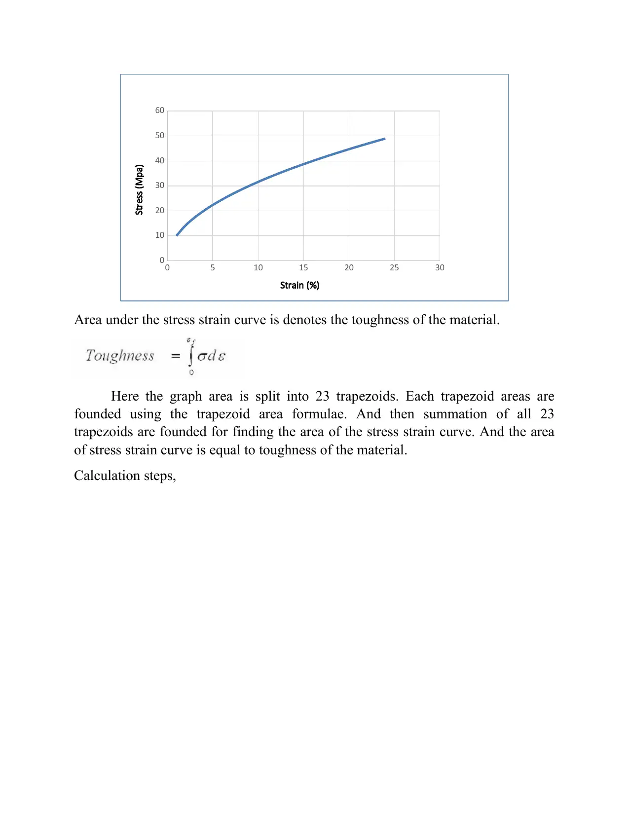
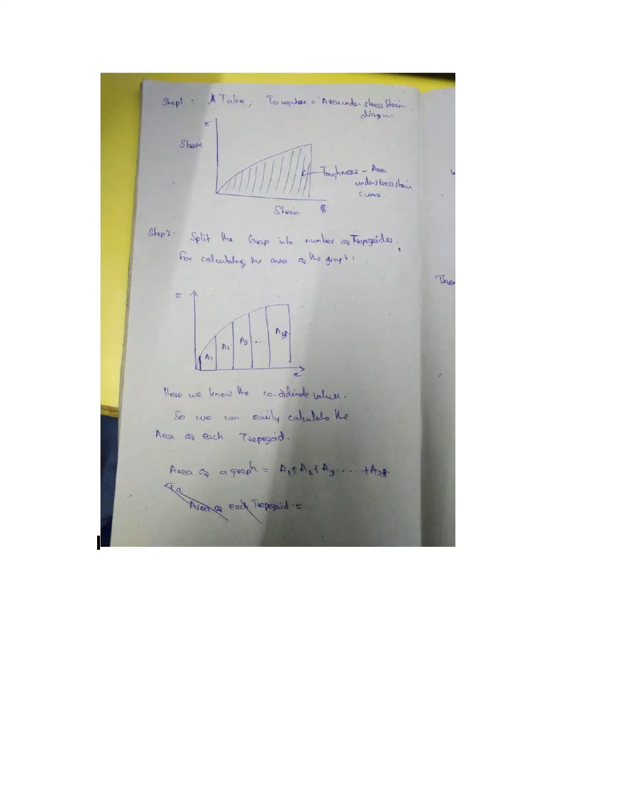
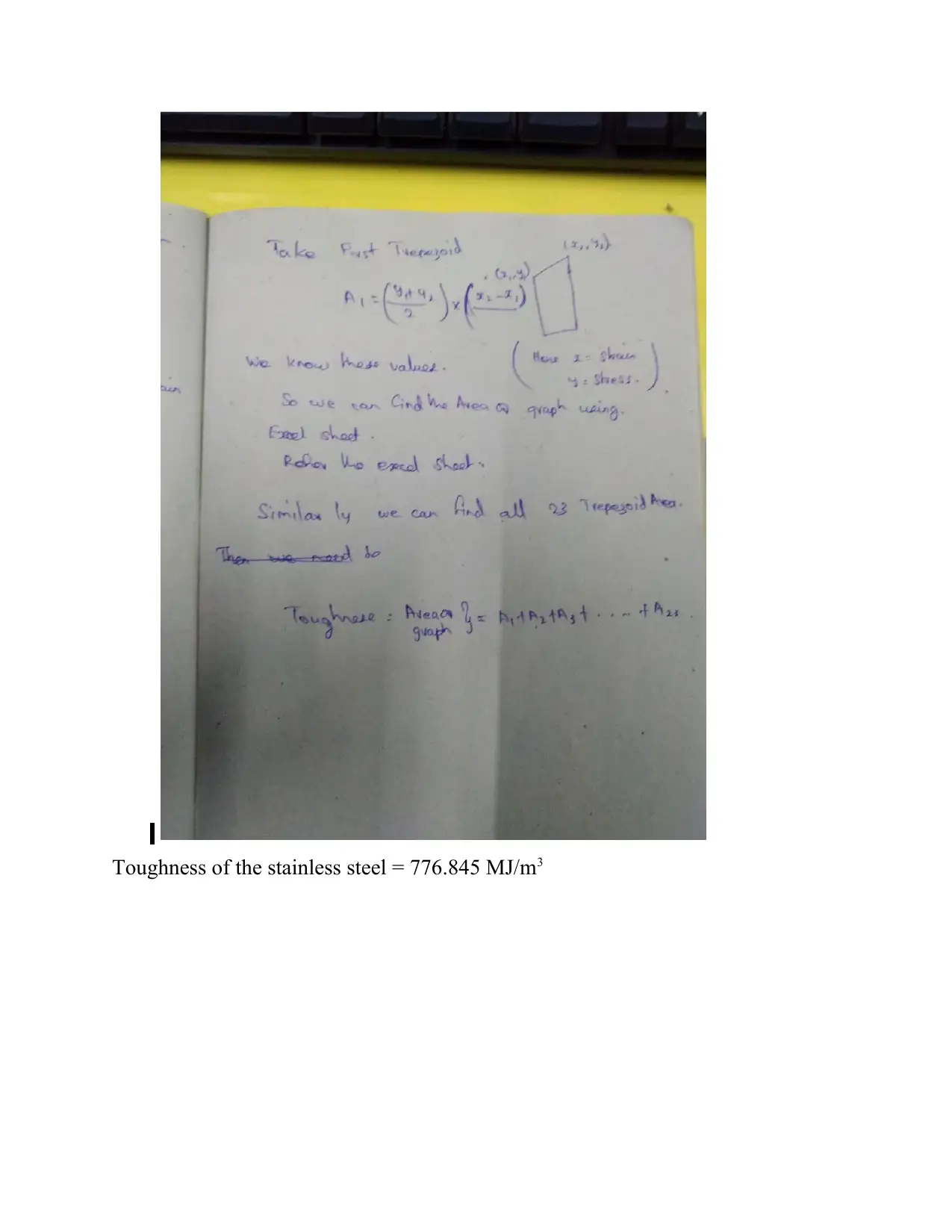
Area under the stress strain curve is denotes the toughness of the material.
Here the graph area is split into 23 trapezoids. Each trapezoid areas are
founded using the trapezoid area formulae. And then summation of all 23
trapezoids are founded for finding the area of the stress strain curve. And the area
of stress strain curve is equal to toughness of the material.
Calculation steps,

Toughness of the stainless steel = 776.845 MJ/m3

Investigation 4: Quality Control (25%)
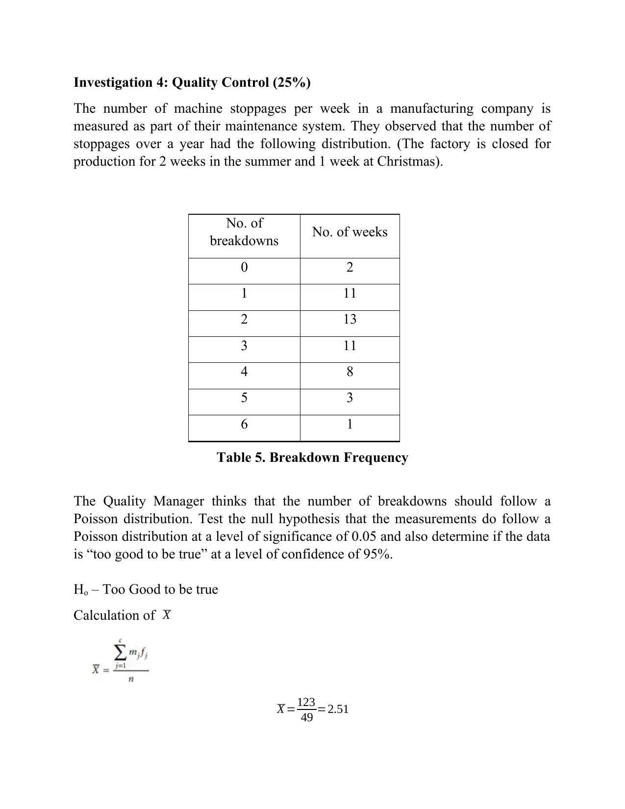
The number of machine stoppages per week in a manufacturing company is
measured as part of their maintenance system. They observed that the number of
stoppages over a year had the following distribution. (The factory is closed for
production for 2 weeks in the summer and 1 week at Christmas).
No. of
breakdowns No. of weeks
0 2
1 11
2 13
3 11
4 8
5 3
6 1
Table 5. Breakdown Frequency
The Quality Manager thinks that the number of breakdowns should follow a
Poisson distribution. Test the null hypothesis that the measurements do follow a
Poisson distribution at a level of significance of 0.05 and also determine if the data
is “too good to be true” at a level of confidence of 95%.
Ho – Too Good to be true
Calculation of X
X =123
49 =2.51

Probability value founded from the below given formula.
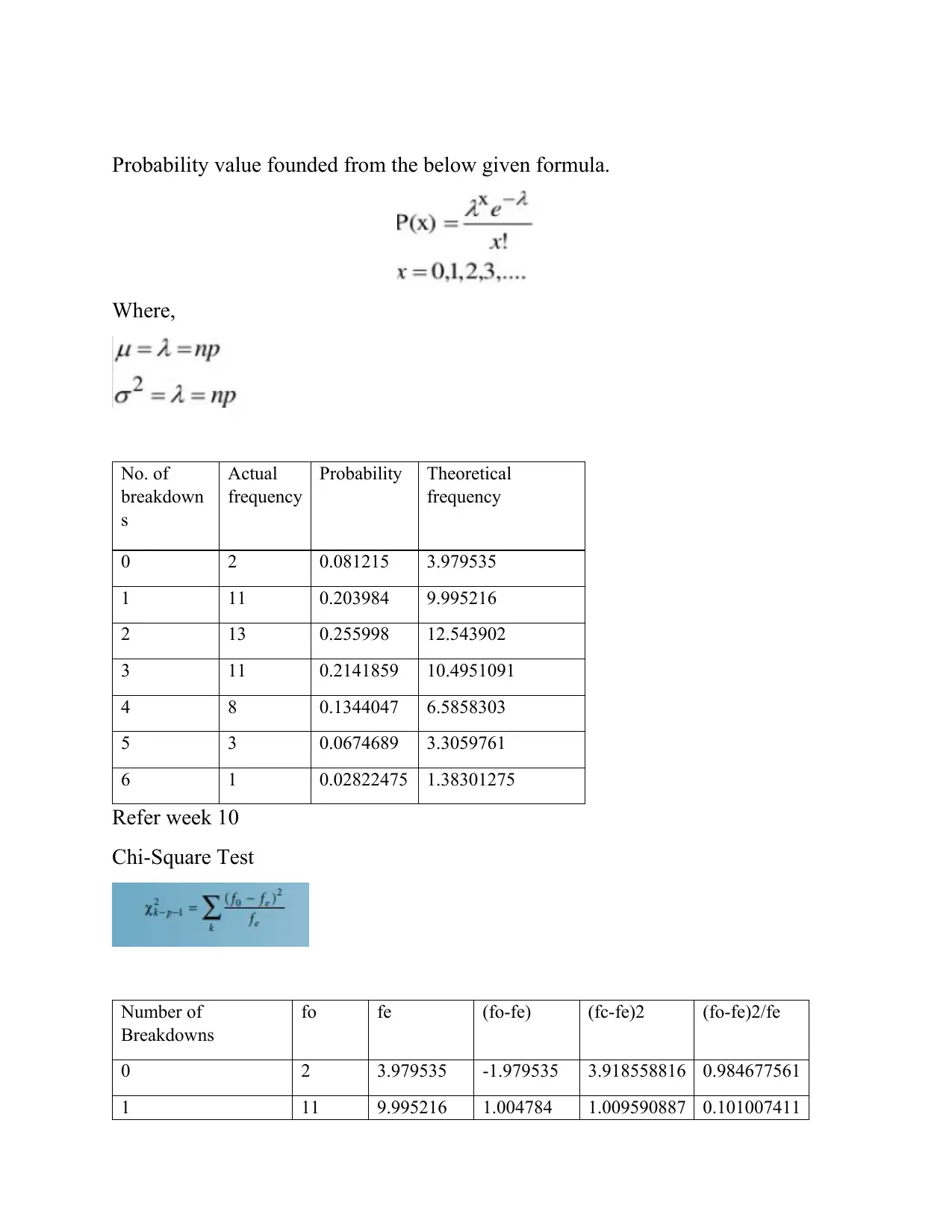
Where,
No. of
breakdown
s
Actual
frequency
Probability Theoretical
frequency
0 2 0.081215 3.979535
1 11 0.203984 9.995216
2 13 0.255998 12.543902
3 11 0.2141859 10.4951091
4 8 0.1344047 6.5858303
5 3 0.0674689 3.3059761
6 1 0.02822475 1.38301275
Refer week 10
Chi-Square Test
Number of
Breakdowns
fo fe (fo-fe) (fc-fe)2 (fo-fe)2/fe
0 2 3.979535 -1.979535 3.918558816 0.984677561
1 11 9.995216 1.004784 1.009590887 0.101007411

2 13 12.543902 0.456098 0.208025386 0.016583786
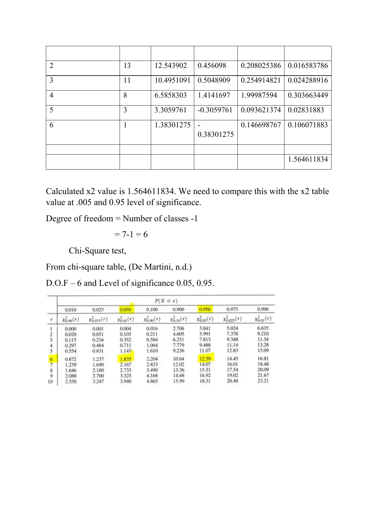
3 11 10.4951091 0.5048909 0.254914821 0.024288916
4 8 6.5858303 1.4141697 1.99987594 0.303663449
5 3 3.3059761 -0.3059761 0.093621374 0.02831883
6 1 1.38301275 -
0.38301275
0.146698767 0.106071883
1.564611834
Calculated x2 value is 1.564611834. We need to compare this with the x2 table
value at .005 and 0.95 level of significance.
Degree of freedom = Number of classes -1
= 7-1 = 6
Chi-Square test,
From chi-square table, (De Martini, n.d.)
D.O.F – 6 and Level of significance 0.05, 0.95.

Chi-Square value at 0.05 level of significance = 1.635
Chi-Square value at 0.05 level of significance = 12.59
X20.05 > X2calculated
X20.95 > X2Calculated.
Calculated chi-square value not present in the boundary condition. And also it
smaller than X20.05. So accept null hypothesis. And the null hypothesis is too good
to be true.

References
Cain, T. (2007). Spring design & manufacture. Poole, Dorset, England: Special
Interest Model Books.
De Martini, D. (n.d.). Success probability estimation with applications to clinical
trials.
Kumar, A. and Shah, G. (2010). Thermal engineering. Oxford: Alpha Science
International.