Advanced Thermal and Fluid Engineering
VerifiedAdded on 2022/12/27
|17
|2546
|43
AI Summary
This document discusses two problems in advanced thermal and fluid engineering. The first problem involves solving a simple initial value problem using the finite difference method. The second problem focuses on solving a one-dimensional convection diffusion problem. MATLAB code is provided for both problems.
Contribute Materials
Your contribution can guide someone’s learning journey. Share your
documents today.
Running head: ADVANCED THERMAL AND FLUID ENGINEERING
ADVANCED THERMAL AND FLUID ENGINEERING
Name of the Student
Name of the University
Author Note
ADVANCED THERMAL AND FLUID ENGINEERING
Name of the Student
Name of the University
Author Note
Secure Best Marks with AI Grader
Need help grading? Try our AI Grader for instant feedback on your assignments.
1ADVANCED THERMAL AND FLUID ENGINEERING
Part one: Simple initial value problem
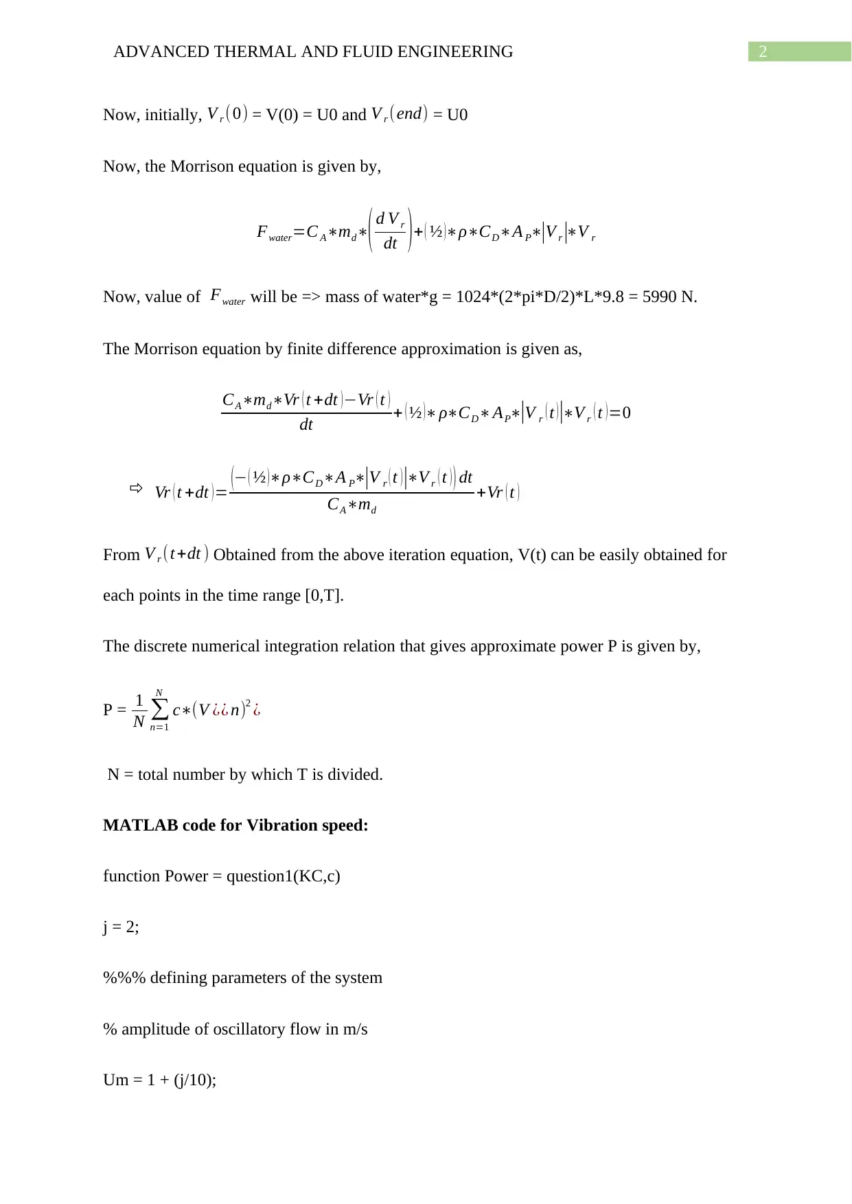
In this particular task the equation of motion of a cylinder through which water flows in a
variable rate is modelled and then the vibration of the cylinder is obtained by numeric
solution by FDM approach. The energy extracted by the electricity is obtained from the
power generated though the vibration of the cylinder. This is modelled by a damper with a
certain damping constant c and a spring with spring constant k as shown in the figure below.
Last digit of student id is j = 2
Given, Um= 1 + 2/10 = 1.2 m/s, U0 = 0.1*1.2 = 0.12 m/s, D = 10 + 2 = 12 cm = 12*10^(-2)
m, Mass of cylinder m = 50 kgs, Water density ρ = 1024 kg/m^3, Stiffness of spring K = 200
N/m, Damping coefficient c = 10 N*m/sec, md = 1 and CA = CD = 1.
The KC number is given by,
KC = Um*T/D
Hence, for KC = 2 => T = 2*D/Um = 0.2 sec.
The entire time of 0.2 sec is divided in small steps.
Flow velocity V r =u−V
Part one: Simple initial value problem
In this particular task the equation of motion of a cylinder through which water flows in a
variable rate is modelled and then the vibration of the cylinder is obtained by numeric
solution by FDM approach. The energy extracted by the electricity is obtained from the
power generated though the vibration of the cylinder. This is modelled by a damper with a
certain damping constant c and a spring with spring constant k as shown in the figure below.
Last digit of student id is j = 2
Given, Um= 1 + 2/10 = 1.2 m/s, U0 = 0.1*1.2 = 0.12 m/s, D = 10 + 2 = 12 cm = 12*10^(-2)
m, Mass of cylinder m = 50 kgs, Water density ρ = 1024 kg/m^3, Stiffness of spring K = 200
N/m, Damping coefficient c = 10 N*m/sec, md = 1 and CA = CD = 1.
The KC number is given by,
KC = Um*T/D
Hence, for KC = 2 => T = 2*D/Um = 0.2 sec.
The entire time of 0.2 sec is divided in small steps.
Flow velocity V r =u−V
2ADVANCED THERMAL AND FLUID ENGINEERING
Now, initially, V r (0) = V(0) = U0 and V r (end) = U0
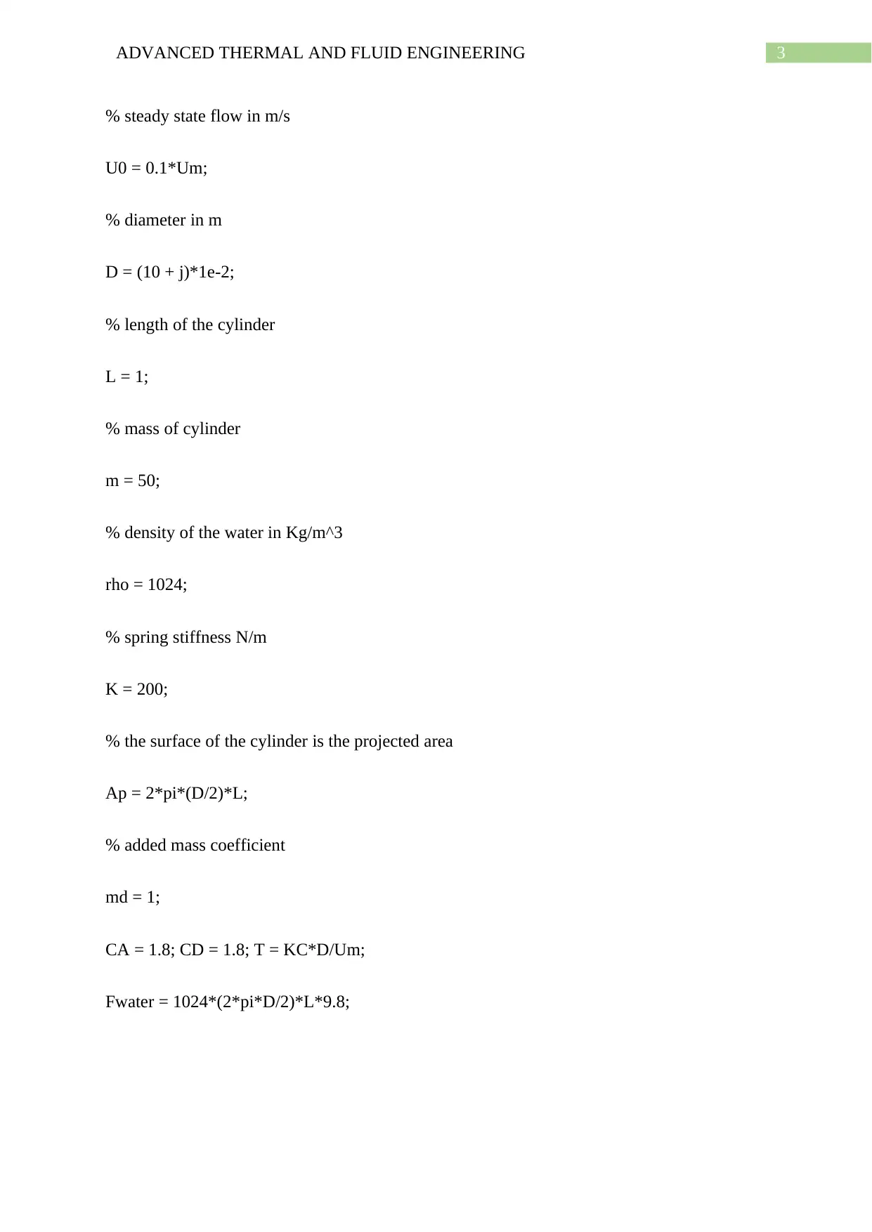
Now, the Morrison equation is given by,
Fwater=C A∗md∗( d V r
dt )+ ( ½ )∗ρ∗CD∗A P∗|V r |∗V r
Now, value of Fwater will be => mass of water*g = 1024*(2*pi*D/2)*L*9.8 = 5990 N.
The Morrison equation by finite difference approximation is given as,
CA∗md∗Vr ( t +dt ) −Vr ( t )
dt + ( ½ )∗ρ∗CD∗AP∗|V r ( t )|∗V r ( t ) =0
Vr ( t +dt )= (− ( ½ )∗ρ∗CD∗A P∗|V r ( t )|∗V r ( t ) ) dt
CA∗md
+Vr ( t )
From V r (t+dt ) Obtained from the above iteration equation, V(t) can be easily obtained for
each points in the time range [0,T].
The discrete numerical integration relation that gives approximate power P is given by,
P = 1
N ∑
n=1
N
c∗(V ¿¿ n)2 ¿
N = total number by which T is divided.
MATLAB code for Vibration speed:
function Power = question1(KC,c)
j = 2;
%%% defining parameters of the system
% amplitude of oscillatory flow in m/s
Um = 1 + (j/10);
Now, initially, V r (0) = V(0) = U0 and V r (end) = U0
Now, the Morrison equation is given by,
Fwater=C A∗md∗( d V r
dt )+ ( ½ )∗ρ∗CD∗A P∗|V r |∗V r
Now, value of Fwater will be => mass of water*g = 1024*(2*pi*D/2)*L*9.8 = 5990 N.
The Morrison equation by finite difference approximation is given as,
CA∗md∗Vr ( t +dt ) −Vr ( t )
dt + ( ½ )∗ρ∗CD∗AP∗|V r ( t )|∗V r ( t ) =0
Vr ( t +dt )= (− ( ½ )∗ρ∗CD∗A P∗|V r ( t )|∗V r ( t ) ) dt
CA∗md
+Vr ( t )
From V r (t+dt ) Obtained from the above iteration equation, V(t) can be easily obtained for
each points in the time range [0,T].
The discrete numerical integration relation that gives approximate power P is given by,
P = 1
N ∑
n=1
N
c∗(V ¿¿ n)2 ¿
N = total number by which T is divided.
MATLAB code for Vibration speed:
function Power = question1(KC,c)
j = 2;
%%% defining parameters of the system
% amplitude of oscillatory flow in m/s
Um = 1 + (j/10);
3ADVANCED THERMAL AND FLUID ENGINEERING
% steady state flow in m/s
U0 = 0.1*Um;
% diameter in m
D = (10 + j)*1e-2;
% length of the cylinder
L = 1;
% mass of cylinder
m = 50;
% density of the water in Kg/m^3
rho = 1024;
% spring stiffness N/m
K = 200;
% the surface of the cylinder is the projected area
Ap = 2*pi*(D/2)*L;
% added mass coefficient
md = 1;
CA = 1.8; CD = 1.8; T = KC*D/Um;
Fwater = 1024*(2*pi*D/2)*L*9.8;
Secure Best Marks with AI Grader
Need help grading? Try our AI Grader for instant feedback on your assignments.

4ADVANCED THERMAL AND FLUID ENGINEERING
t = linspace(0,T,150);
dt = t(2)- t(1);
Vr = U0 + Um.*sin(2*pi*t/T);
Vr(1) = U0; Vr(end) = U0;
%%% solving Vr(t) by FDM
for incdt = 2:length(t)-2
Vr(incdt+1) = (- (1/2)*rho*CD*Ap*abs(Vr(incdt))*Vr(incdt))*dt/(CA*md) + Vr(incdt);
end
V = Vr;
plot(t,V,'b-')
xlabel('Time t in secs')
ylabel('Vibration speed in m/sec')
title('Vibration speed Vs time')
grid on
%%% computing Power extracted P from electricity generator
Power=0;
5ADVANCED THERMAL AND FLUID ENGINEERING
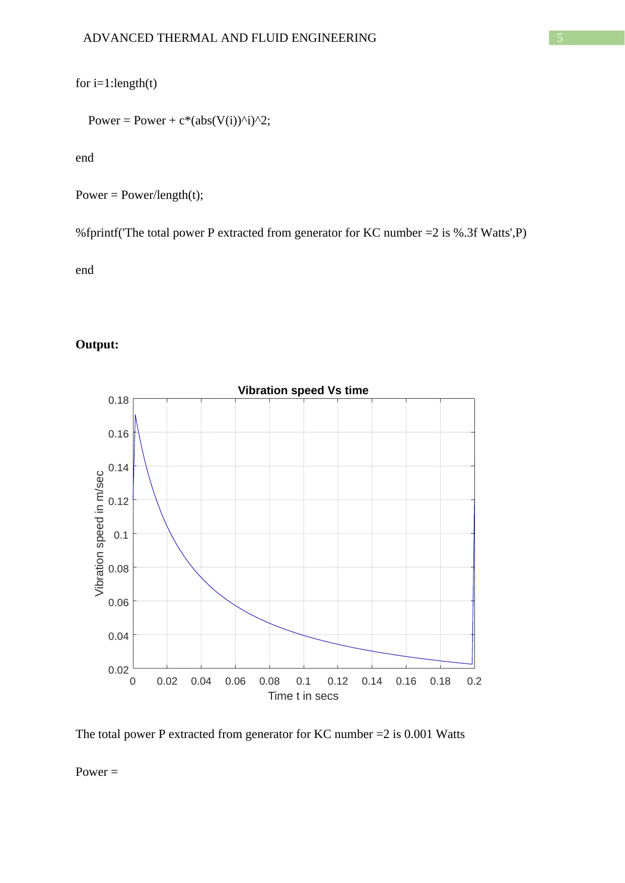
for i=1:length(t)
Power = Power + c*(abs(V(i))^i)^2;
end
Power = Power/length(t);
%fprintf('The total power P extracted from generator for KC number =2 is %.3f Watts',P)
end
Output:
0 0.02 0.04 0.06 0.08 0.1 0.12 0.14 0.16 0.18 0.2
Time t in secs
0.02
0.04
0.06
0.08
0.1
0.12
0.14
0.16
0.18
Vibration speed in m/sec
Vibration speed Vs time
The total power P extracted from generator for KC number =2 is 0.001 Watts
Power =

6ADVANCED THERMAL AND FLUID ENGINEERING
0.0010
Now, for finding the relationship between KC number and power the MATLAB code is
modified and code for graph generation is given below.
Now, in order to find the power vs KC number relationship the following code is written in
MATLAB.
MATLAB code:
KC = 2:2:20; % KC number range
c= 100; % damping coeffcient in N*m/sec
for i=1:length(KC)
Power(i) = question1(KC(i),c); % Calling function to calculate power at a particular KC
end
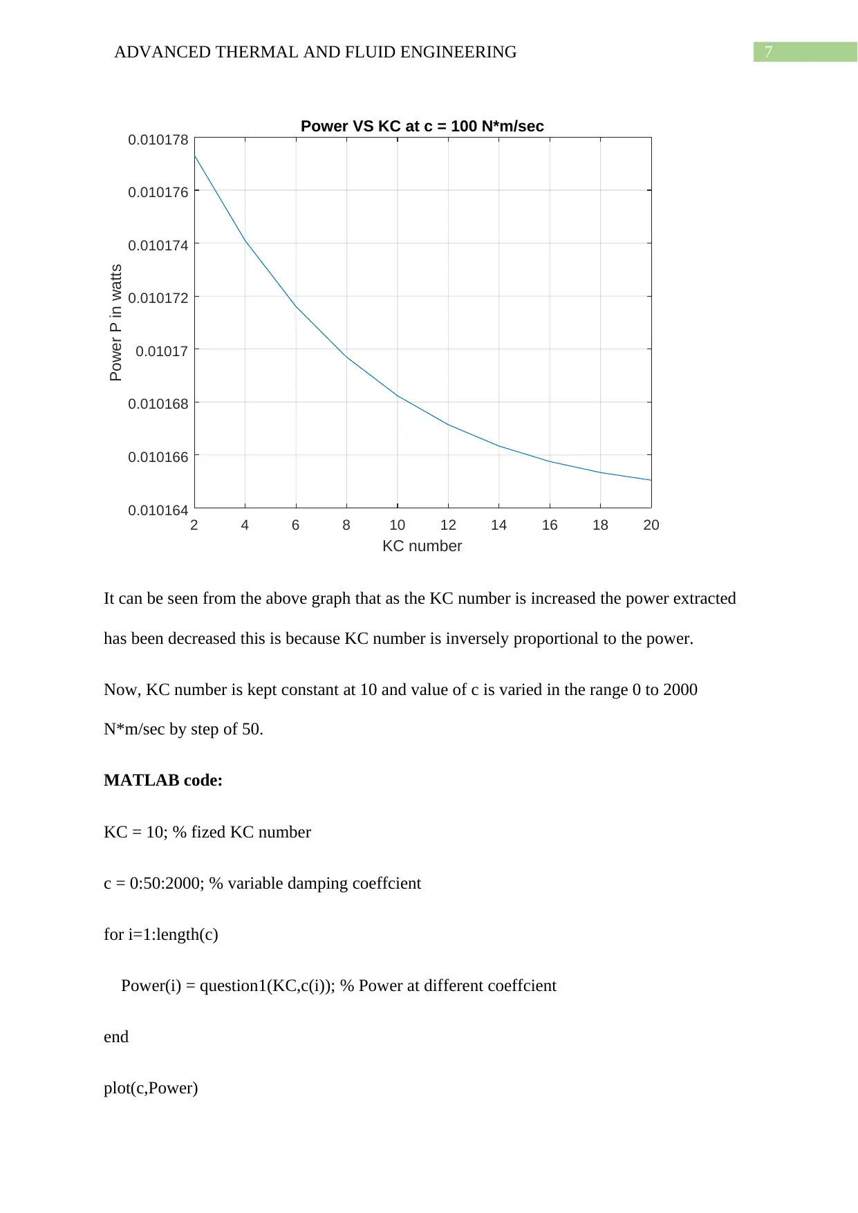
plot(KC,Power)
xlabel('KC number')
ylabel('Power P in watts')
grid on
title('Power VS KC at c = 100 N*m/sec')
Plot:
0.0010
Now, for finding the relationship between KC number and power the MATLAB code is
modified and code for graph generation is given below.
Now, in order to find the power vs KC number relationship the following code is written in
MATLAB.
MATLAB code:
KC = 2:2:20; % KC number range
c= 100; % damping coeffcient in N*m/sec
for i=1:length(KC)
Power(i) = question1(KC(i),c); % Calling function to calculate power at a particular KC
end
plot(KC,Power)
xlabel('KC number')
ylabel('Power P in watts')
grid on
title('Power VS KC at c = 100 N*m/sec')
Plot:
Paraphrase This Document
Need a fresh take? Get an instant paraphrase of this document with our AI Paraphraser
7ADVANCED THERMAL AND FLUID ENGINEERING
2 4 6 8 10 12 14 16 18 20
KC number
0.010164
0.010166
0.010168
0.01017
0.010172
0.010174
0.010176
0.010178
Power P in watts
Power VS KC at c = 100 N*m/sec
It can be seen from the above graph that as the KC number is increased the power extracted
has been decreased this is because KC number is inversely proportional to the power.
Now, KC number is kept constant at 10 and value of c is varied in the range 0 to 2000
N*m/sec by step of 50.
MATLAB code:
KC = 10; % fized KC number
c = 0:50:2000; % variable damping coeffcient
for i=1:length(c)
Power(i) = question1(KC,c(i)); % Power at different coeffcient
end
plot(c,Power)
8ADVANCED THERMAL AND FLUID ENGINEERING
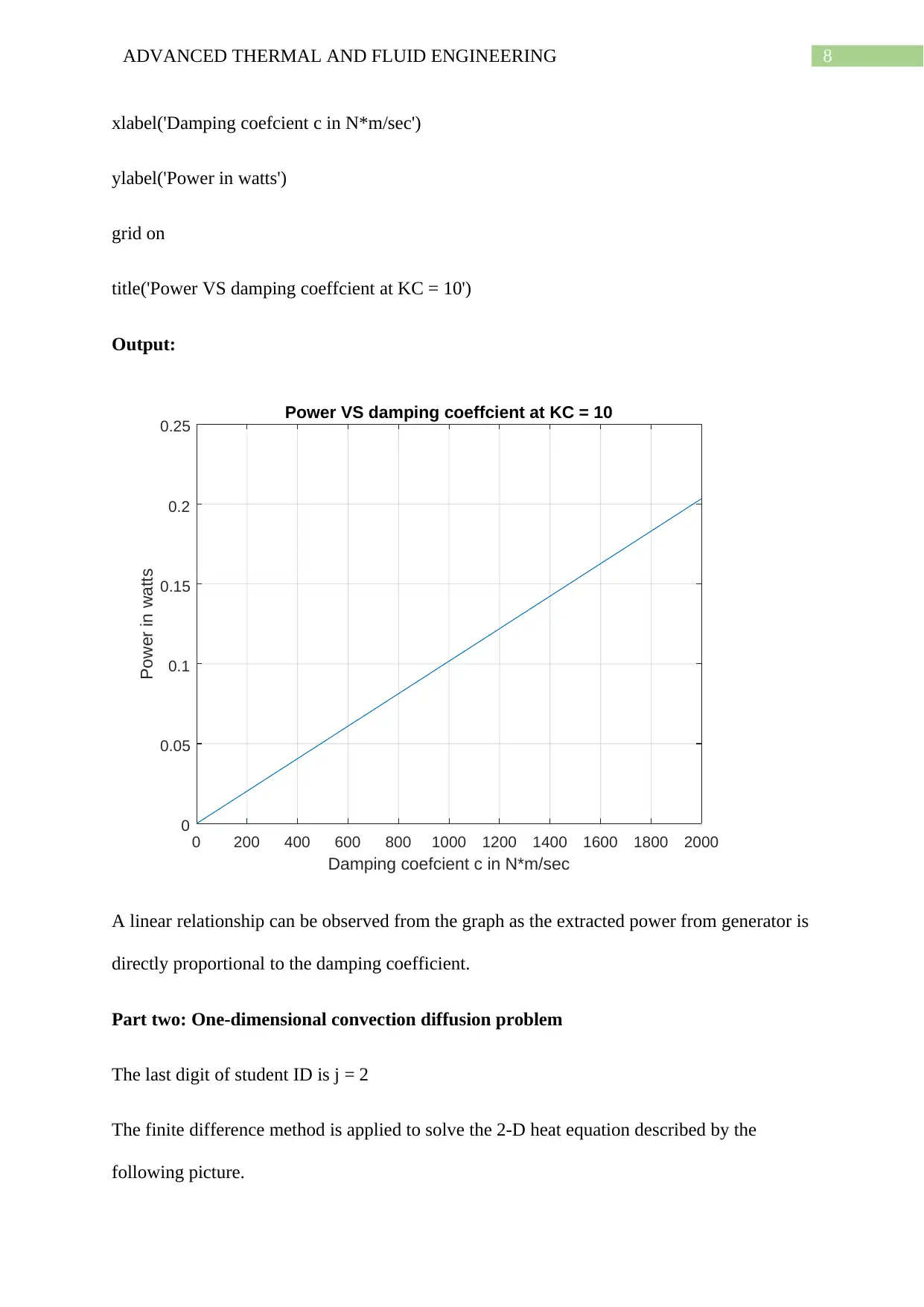
xlabel('Damping coefcient c in N*m/sec')
ylabel('Power in watts')
grid on
title('Power VS damping coeffcient at KC = 10')
Output:
0 200 400 600 800 1000 1200 1400 1600 1800 2000
Damping coefcient c in N*m/sec
0
0.05
0.1
0.15
0.2
0.25
Power in watts
Power VS damping coeffcient at KC = 10
A linear relationship can be observed from the graph as the extracted power from generator is
directly proportional to the damping coefficient.
Part two: One-dimensional convection diffusion problem
The last digit of student ID is j = 2
The finite difference method is applied to solve the 2-D heat equation described by the
following picture.
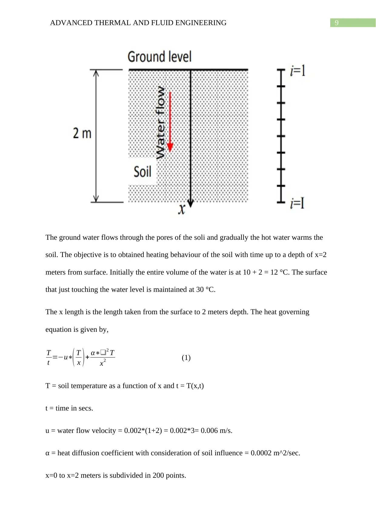
9ADVANCED THERMAL AND FLUID ENGINEERING
The ground water flows through the pores of the soli and gradually the hot water warms the
soil. The objective is to obtained heating behaviour of the soil with time up to a depth of x=2
meters from surface. Initially the entire volume of the water is at 10 + 2 = 12 °C. The surface
that just touching the water level is maintained at 30 °C.
The x length is the length taken from the surface to 2 meters depth. The heat governing
equation is given by,
T
t =−u∗( T
x )+ α∗❑2 T
x2 (1)
T = soil temperature as a function of x and t = T(x,t)
t = time in secs.
u = water flow velocity = 0.002*(1+2) = 0.002*3= 0.006 m/s.
α = heat diffusion coefficient with consideration of soil influence = 0.0002 m^2/sec.
x=0 to x=2 meters is subdivided in 200 points.
Secure Best Marks with AI Grader
Need help grading? Try our AI Grader for instant feedback on your assignments.
10ADVANCED THERMAL AND FLUID ENGINEERING
x= 0 = 1st cell and
x= 2 = 200th cell.
Hence, by finite difference approximation the differential equation (1) becomes
T ( x , t +1 ) – T ( x ,t )
dt =−u∗T ( x +1 , t ) – T ( x , t )
dx + α∗T ( x +1 ,t ) – 2∗T ( x , t ) + T ( x−1 ,t )
d x2
OR,
T ( x , t+1 ) = ( −u∗T ( x+1 , t ) – T ( x , t )
dx + α∗T ( x +1 , t ) – 2∗T ( x ,t ) +T ( x−1 , t )
d x2 )∗dt +T (x , t)
Variation of temperature = i-1 to i+1 cells
Where, i-1 to i+1 varies from temperature at 1st to 200th cell or point.
Boundary conditions are T|x=0 = 30 °C, T
x =0 at x= 2.
Also, T(i) = (10 + j) = (10+2) °C = 12 °C initially.
T
x =0 at x= 2 => (T(200,t) – T(199,t))/dx = 0
Hence, T(200,t) = T(199,t) Or, T(200,t) = T(199,t)
Hence, by finite difference method temperatures from T(1) to T(199) is calculated and then
the value of T(199) is made equal to T(200).
MATLAB code for temperature plot and T1.5 at α = 0.0002 m^2/sec:
function time25 = question2(alpha) % coeffcient of heat diffusion in m^2/sec
j=2;
% flow velocity
11ADVANCED THERMAL AND FLUID ENGINEERING
u = 0.002*(1+j);
% dividing 0 to 2 meters
x= linspace(0,2,200);
% step increment of x
dx = x(2) - x(1);
% unit increment of time
dt = 2*dx;
% 0 to 300 secs
t = 0:dt:300;
% initial temperature is 12 degree C
initialT = 10+j;
% initially T is at 12 degree C for all t and x
Temp = repmat(initialT,length(x),length(t));
% applying boundary conditions
Temp(1,:) = 30; Temp(199,:) = Temp(200,:);
for incdt = 1:length(t)-1
for incdx = 2:length(x)-1

12ADVANCED THERMAL AND FLUID ENGINEERING
Temp(incdx,incdt+1) = dt*(-u*(Temp(incdx+1,incdt) - Temp(incdx,incdt))/dx +
alpha*(Temp(incdx+1,incdt) - 2*Temp(incdx,incdt) + Temp(incdx-1,incdt))/dx^2) +
Temp(incdx,incdt); % FDM iteration equation
end
end
Temp(200,:) = Temp(199,:);
% [xx,tt] = meshgrid(x,t);
% mesh(xx,tt,T')
% xlabel('Depth in [0,2] m')
% ylabel('Time in Sec')
% zlabel('Temperature in Degree C')
% title('Temperature plot T(x,t)')
% grid on
for i=1:length(x)
if round(x(i),2) == 1.51
xlen = i;
else
end
Paraphrase This Document
Need a fresh take? Get an instant paraphrase of this document with our AI Paraphraser
13ADVANCED THERMAL AND FLUID ENGINEERING
end
T25 = Temp(xlen,:);
for j=1:length(T25)
if round(T25(j),1) == 25
Tpos = j;
else
end
end
%fprintf('At x=1.5 m, the temperature is approximately 25 degree C at time t= %.3f secs \
n',t(Tpos)) % Displaying time to reach 25 degree C of the length x=1.5 m
time25 = t(Tpos);
end
Output:
end
T25 = Temp(xlen,:);
for j=1:length(T25)
if round(T25(j),1) == 25
Tpos = j;
else
end
end
%fprintf('At x=1.5 m, the temperature is approximately 25 degree C at time t= %.3f secs \
n',t(Tpos)) % Displaying time to reach 25 degree C of the length x=1.5 m
time25 = t(Tpos);
end
Output:
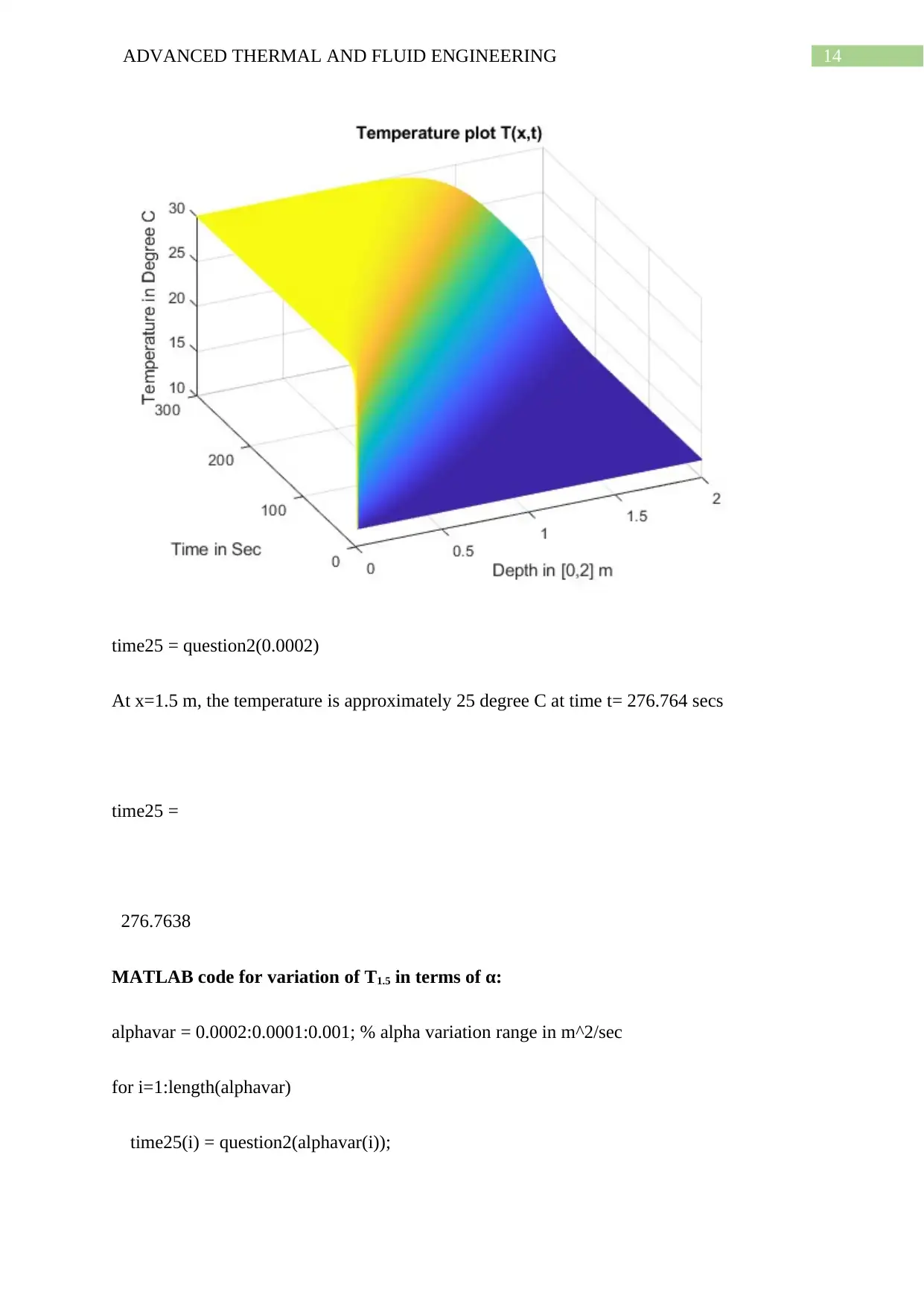
14ADVANCED THERMAL AND FLUID ENGINEERING
time25 = question2(0.0002)
At x=1.5 m, the temperature is approximately 25 degree C at time t= 276.764 secs
time25 =
276.7638
MATLAB code for variation of T1.5 in terms of α:
alphavar = 0.0002:0.0001:0.001; % alpha variation range in m^2/sec
for i=1:length(alphavar)
time25(i) = question2(alphavar(i));
15ADVANCED THERMAL AND FLUID ENGINEERING
end
plot(alphavar,time25)
xlabel('variation of heat diffusion coefficient \alpha in m^2/sec')
ylabel('Time to reach 1.5 m depth to 25 degree C in secs')
title('\alpha VS T_{1.5}')
grid on
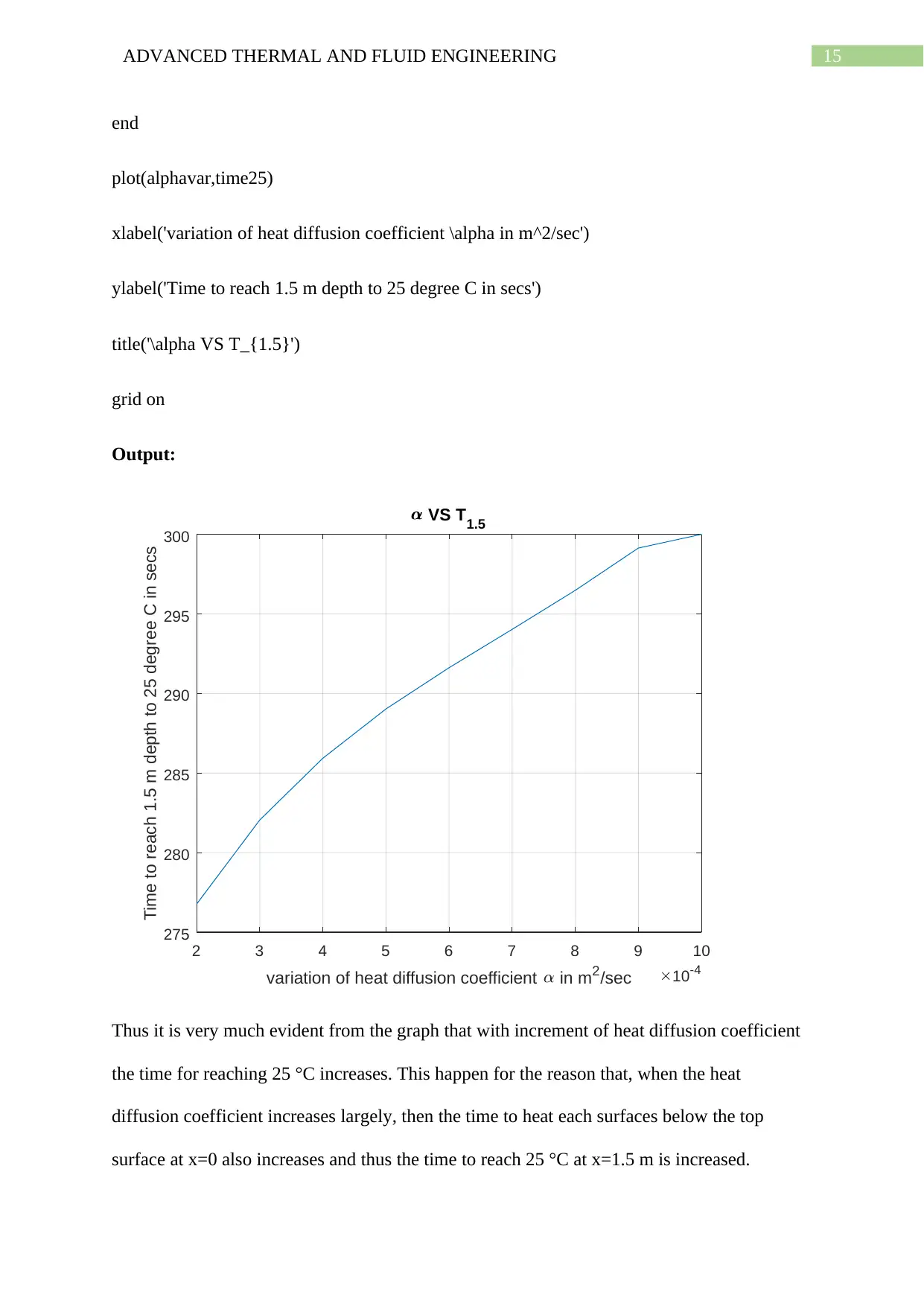
Output:
2 3 4 5 6 7 8 9 10
variation of heat diffusion coefficient in m2/sec 10-4
275
280
285
290
295
300
Time to reach 1.5 m depth to 25 degree C in secs
VS T1.5
Thus it is very much evident from the graph that with increment of heat diffusion coefficient
the time for reaching 25 °C increases. This happen for the reason that, when the heat
diffusion coefficient increases largely, then the time to heat each surfaces below the top
surface at x=0 also increases and thus the time to reach 25 °C at x=1.5 m is increased.
end
plot(alphavar,time25)
xlabel('variation of heat diffusion coefficient \alpha in m^2/sec')
ylabel('Time to reach 1.5 m depth to 25 degree C in secs')
title('\alpha VS T_{1.5}')
grid on
Output:
2 3 4 5 6 7 8 9 10
variation of heat diffusion coefficient in m2/sec 10-4
275
280
285
290
295
300
Time to reach 1.5 m depth to 25 degree C in secs
VS T1.5
Thus it is very much evident from the graph that with increment of heat diffusion coefficient
the time for reaching 25 °C increases. This happen for the reason that, when the heat
diffusion coefficient increases largely, then the time to heat each surfaces below the top
surface at x=0 also increases and thus the time to reach 25 °C at x=1.5 m is increased.
Secure Best Marks with AI Grader
Need help grading? Try our AI Grader for instant feedback on your assignments.

16ADVANCED THERMAL AND FLUID ENGINEERING
1 out of 17
Related Documents


Your All-in-One AI-Powered Toolkit for Academic Success.
+13062052269
info@desklib.com
Available 24*7 on WhatsApp / Email
![[object Object]](/_next/static/media/star-bottom.7253800d.svg)
Unlock your academic potential
© 2024 | Zucol Services PVT LTD | All rights reserved.