AFIN 102 | S2 2019 Individual Assignment 2022

AFIN 102 | S2 2019 | Individual Assignment
Student Number:
AFIN 102 Individual Assignment Report
Executive Summary
Assigned
Company Name Eagerengineering
Sector Finance brokerage company
10/9/2019 Page 1 of
14

AFIN 102 | S2 2019 | Individual Assignment
Student Number:
Executive summary
The report brings out a discussion on brokerage companies in Australia. The report has a comparison
on Eagerengineering (service provider in Australia) with other same companies listed on ASX. It has
been reported that the Sydney based brokerage organisation has been significantly growing in the last
few years (Pontusson, and Weisstanner, 2018). The two competitors selected for analysis and
comparison are Shore financial, which has built $1.85 billion loan amount under the last five years.
For another competitor, it is seen that Aussie is selected that engages 1018 brokers and total loan of $
68,883,900,000 (Ermilova, and Finogenova, 2017). The report will discuss on the performance of the
industry for five years, DCF model has been used for the valuation purpose for EagerEngineering
with the assistance of some financial ratios. Comparable P/E ratio has been used to estimate the share
price of EageraEngineering based on price/EBITDA, P/E to Growth, Price to Sales and Enterprise
Value/EBITDA (The Adviser, 2018).
Macroeconomic and Industry Analysis
The consumer market of Australia is marked at 15th rank through household final consumption of
nearly 752260 million US dollars. The brokerage industry data reports reveal that the revenue of the
industry has increased for the last five years with the increase in consumer preferences, and
insurance premiums (Cornell, and Gokhale, 2015). The data of industry reveals that it has a revenue
of 13 billion dollars, annual growth of 0.3 percent with employee base of 10610 (OECD Economic
Surveys Australia, 2018). Whereas, the investment banking brokerage industry reveals that the
industry income has risen over the time dealing with the increase in volume dealings (Stanford,
Hardy, and Stewart, 2018). The companies has to consider compliance costs, online trading
platforms, performance of the traditional stockbroker, and higher trading volumes (Australian
government, 2016). It states a revenue of 7 billion dollars, 2.9 percent annual growth, employee base
of 15727 (Green, Hand, and Zhang, 2016). The key successful factors revealed for the brokerage
organisations include good reputation, loyal customer base, and accessibility to the niche markets
10/9/2019 Page 2 of
14

AFIN 102 | S2 2019 | Individual Assignment
Student Number:
(Australian government, 2016). Brokers face competition from banks; insurers getting benefits from
threats to the industry outsourced insurance services (OECD Economic Surveys Australia, 2018).
As per the reports of majority of brokerage organisations, it is found that there are risk concerns such
as risk of transfers coverage such as risk of people`s transferring, risk associated with the supply
chain, business interruption, damage of property especially when the company is not aware of
insurance policy (Australian government, 2016). 80 percent of risks are associated with interruption
and risk of supply chain that result into damaging the business confidence and other political
regulation uncertainties (Green, Hand, and Zhang, 2016). Furthermore, changing political landscape,
higher unemployment, corporate governance, lack of skills, and weakening of Australian dollar
presenting the risk environment for company to manage (OECD Economic Surveys Australia, 2018).
In the long term, the organisation suffer from several Macro-economic factors-
Economic factors-
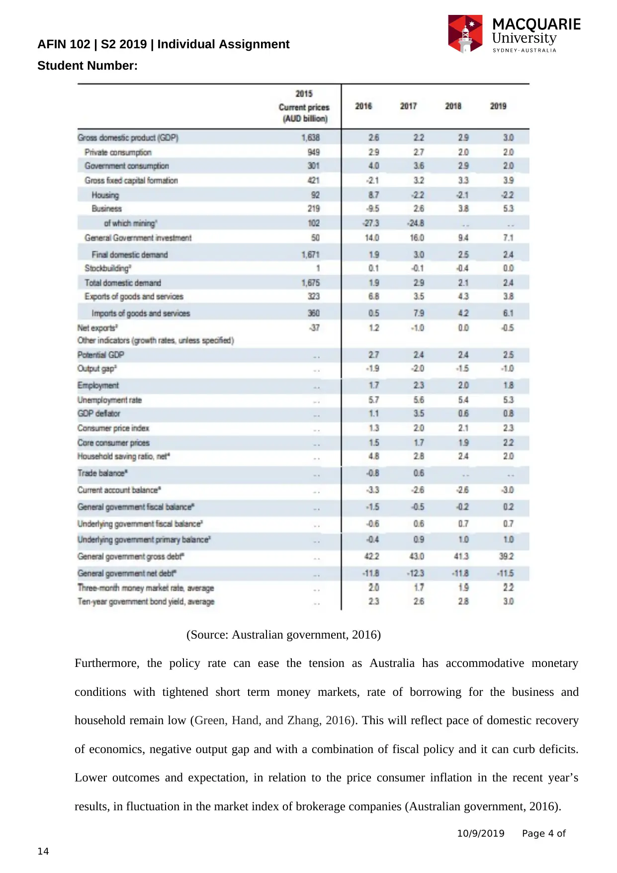
Recent macroeconomic factors will include fiscal policy, monetary policy, economic outputs,
inflation rate, unemployment rate, and economic growth (Cornell, and Gokhale, 2016). The output
growth has been strengthening through rising segment of resource sector with increase in the
resource sector (Green, Hand, and Zhang, 2016). Data depicts that with the increasing knowledge of
share prices and MNCs operations, the investor started to invest in the public sectors. The central
projection growth is estimated at 3 percent in 2018 and 2019 (Australian government, 2016). The
consumer price inflation is in the range of 2 to 3 percent (Green, Hand, and Zhang, 2016). As the
wage growth is quite low, it is seen that weak demand and employment growth is seen. With the
increase and boost employment, it is seen that there the labour force participation can be with a sharp
hike overviewing the labour supply (Cornell, and Gokhale, 2016).
10/9/2019 Page 3 of
14

AFIN 102 | S2 2019 | Individual Assignment
Student Number:
(Source: Australian government, 2016)
Furthermore, the policy rate can ease the tension as Australia has accommodative monetary
conditions with tightened short term money markets, rate of borrowing for the business and
household remain low (Green, Hand, and Zhang, 2016). This will reflect pace of domestic recovery
of economics, negative output gap and with a combination of fiscal policy and it can curb deficits.
Lower outcomes and expectation, in relation to the price consumer inflation in the recent year’s
results, in fluctuation in the market index of brokerage companies (Australian government, 2016).
10/9/2019 Page 4 of
14

AFIN 102 | S2 2019 | Individual Assignment
Student Number:
DCF Analysis
1. Key ratio for DCF analysis
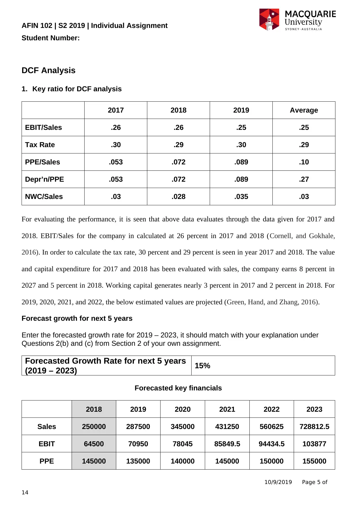
2017 2018 2019 Average
EBIT/Sales .26 .26 .25 .25
Tax Rate .30 .29 .30 .29
PPE/Sales .053 .072 .089 .10
Depr’n/PPE .053 .072 .089 .27
NWC/Sales .03 .028 .035 .03
For evaluating the performance, it is seen that above data evaluates through the data given for 2017 and
2018. EBIT/Sales for the company in calculated at 26 percent in 2017 and 2018 (Cornell, and Gokhale,
2016). In order to calculate the tax rate, 30 percent and 29 percent is seen in year 2017 and 2018. The value
and capital expenditure for 2017 and 2018 has been evaluated with sales, the company earns 8 percent in
2027 and 5 percent in 2018. Working capital generates nearly 3 percent in 2017 and 2 percent in 2018. For
2019, 2020, 2021, and 2022, the below estimated values are projected (Green, Hand, and Zhang, 2016).
Forecast growth for next 5 years
Enter the forecasted growth rate for 2019 – 2023, it should match with your explanation under
Questions 2(b) and (c) from Section 2 of your own assignment.
Forecasted Growth Rate for next 5 years
(2019 – 2023) 15%
Forecasted key financials
2018 2019 2020 2021 2022 2023
Sales 250000 287500 345000 431250 560625 728812.5
EBIT 64500 70950 78045 85849.5 94434.5 103877
PPE 145000 135000 140000 145000 150000 155000
10/9/2019 Page 5 of
14

AFIN 102 | S2 2019 | Individual Assignment
Student Number:
Depreciation 10500 12075 13886.25 15969 18364.5 21119
NWC 7000 10080 14062 7937 15000 15000
10/9/2019 Page 6 of
14

AFIN 102 | S2 2019 | Individual Assignment
Student Number:
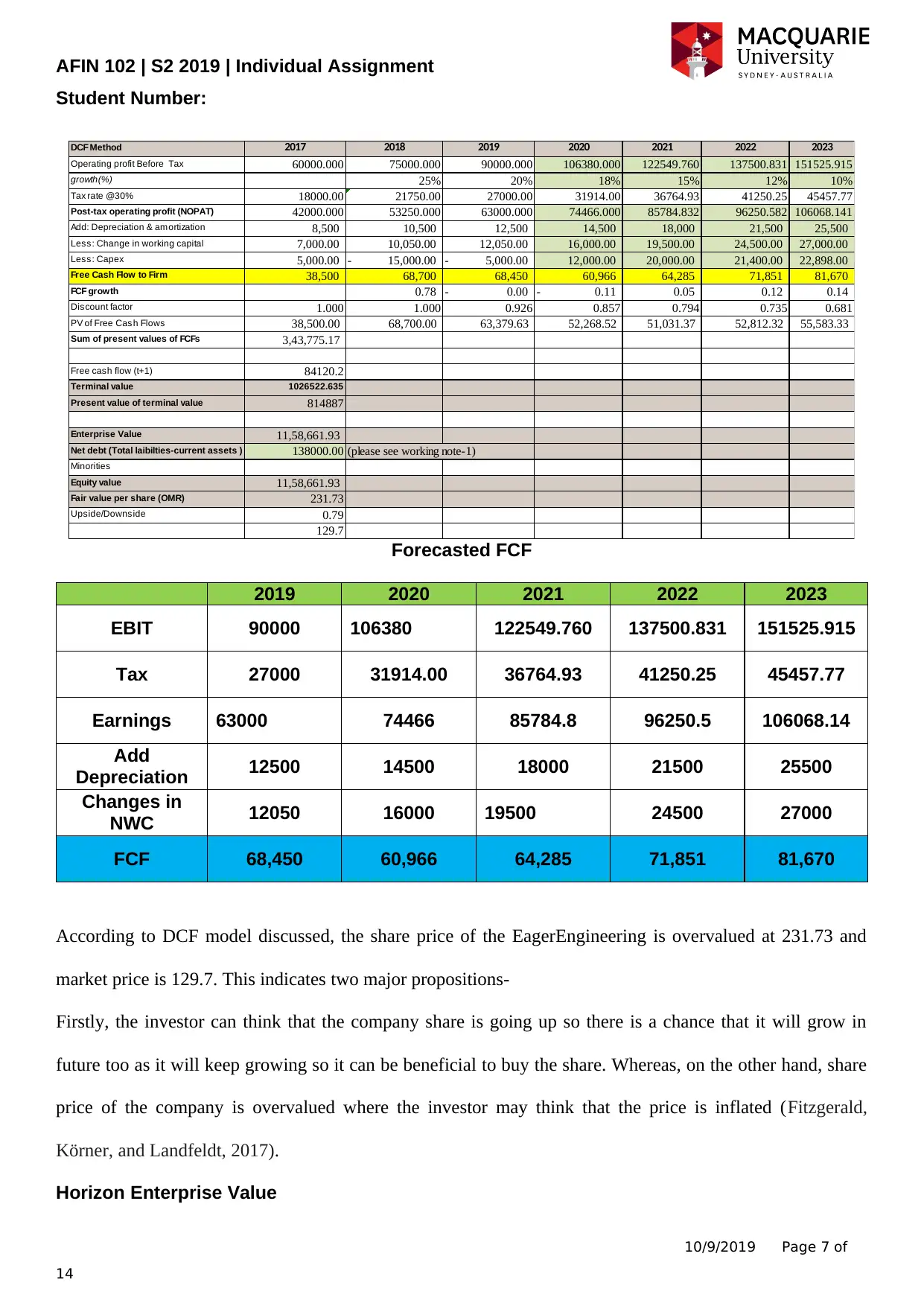
DCF Method 2017 2018 2019 2020 2021 2022 2023
Operating profit Before Tax 60000.000 75000.000 90000.000 106380.000 122549.760 137500.831 151525.915
growth(%) 25% 20% 18% 15% 12% 10%
Tax rate @30% 18000.00 21750.00 27000.00 31914.00 36764.93 41250.25 45457.77
Post-tax operating profit (NOPAT) 42000.000 53250.000 63000.000 74466.000 85784.832 96250.582 106068.141
Add: Depreciation & amortization 8,500 10,500 12,500 14,500 18,000 21,500 25,500
Less: Change in working capital 7,000.00 10,050.00 12,050.00 16,000.00 19,500.00 24,500.00 27,000.00
Less: Capex 5,000.00 15,000.00- 5,000.00- 12,000.00 20,000.00 21,400.00 22,898.00
Free Cash Flow to Firm 38,500 68,700 68,450 60,966 64,285 71,851 81,670
FCF growth 0.78 0.00- 0.11- 0.05 0.12 0.14
Discount factor 1.000 1.000 0.926 0.857 0.794 0.735 0.681
PV of Free Cas h Flows 38,500.00 68,700.00 63,379.63 52,268.52 51,031.37 52,812.32 55,583.33
Sum of present values of FCFs 3,43,775.17
Free cash flow (t+1) 84120.2
Terminal value 1026522.635
Present value of terminal value 814887
Enterprise Value 11,58,661.93
Net debt (Total laibilties-current assets ) 138000.00 (please see working note-1)
Minorities
Equity value 11,58,661.93
Fair value per share (OMR) 231.73
Upside/Downs ide 0.79
129.7
Forecasted FCF
2019 2020 2021 2022 2023
EBIT 90000 106380 122549.760 137500.831 151525.915
Tax 27000 31914.00 36764.93 41250.25 45457.77
Earnings 63000 74466 85784.8 96250.5 106068.14
Add
Depreciation 12500 14500 18000 21500 25500
Changes in
NWC 12050 16000 19500 24500 27000
FCF 68,450 60,966 64,285 71,851 81,670
According to DCF model discussed, the share price of the EagerEngineering is overvalued at 231.73 and
market price is 129.7. This indicates two major propositions-
Firstly, the investor can think that the company share is going up so there is a chance that it will grow in
future too as it will keep growing so it can be beneficial to buy the share. Whereas, on the other hand, share
price of the company is overvalued where the investor may think that the price is inflated (Fitzgerald,
Körner, and Landfeldt, 2017).
Horizon Enterprise Value
10/9/2019 Page 7 of
14

AFIN 102 | S2 2019 | Individual Assignment
Student Number:
Enter the forecasted long-term growth rate beyond 2023, it should match with your explanation
under Question 2(d) from Section 2 of your own assignment.
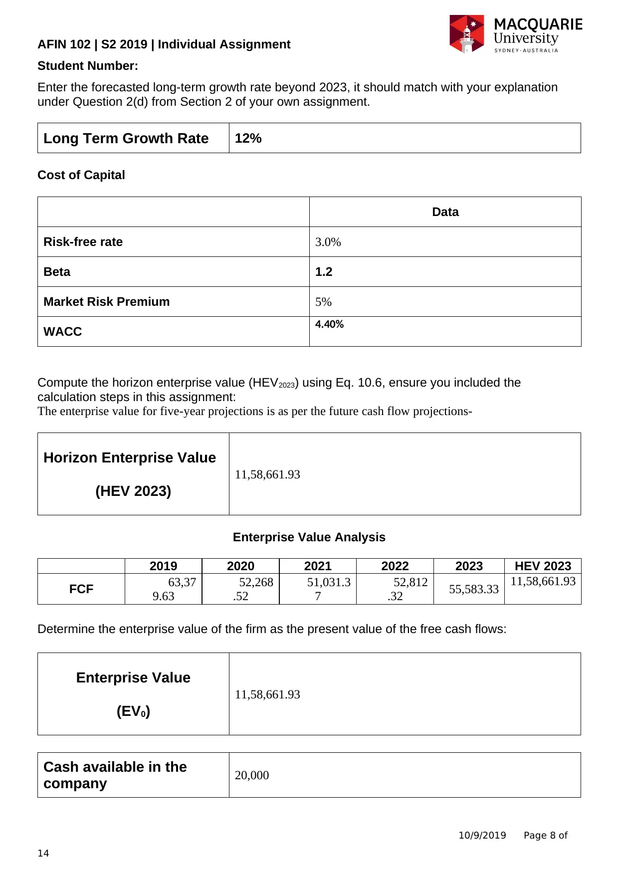
Long Term Growth Rate 12%
Cost of Capital
Data
Risk-free rate 3.0%
Beta 1.2
Market Risk Premium 5%
WACC 4.40%
Compute the horizon enterprise value (HEV2023) using Eq. 10.6, ensure you included the
calculation steps in this assignment:
The enterprise value for five-year projections is as per the future cash flow projections-
Horizon Enterprise Value
(HEV 2023)
11,58,661.93
Enterprise Value Analysis
2019 2020 2021 2022 2023 HEV 2023
FCF 63,37
9.63
52,268
.52
51,031.3
7
52,812
.32 55,583.33 11,58,661.93
Determine the enterprise value of the firm as the present value of the free cash flows:
Enterprise Value
(EV0)
11,58,661.93
Cash available in the
company 20,000
10/9/2019 Page 8 of
14

AFIN 102 | S2 2019 | Individual Assignment
Student Number:
Debt outstanding for the
company 100,000
No. of shares outstanding 5,000
Estimated share price 129.7
10/9/2019 Page 9 of
14

AFIN 102 | S2 2019 | Individual Assignment
Student Number:
Section 4 – Multiple Analysis
1. Companies listed on ASX that is comparable to your allocated company, with explanations and
references:
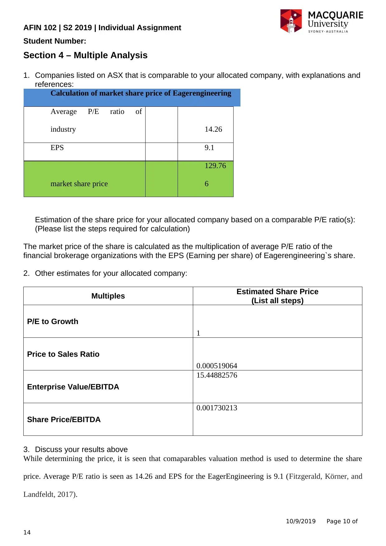
Calculation of market share price of Eagerengineering
Average P/E ratio of
industry 14.26
EPS 9.1
market share price
129.76
6
Estimation of the share price for your allocated company based on a comparable P/E ratio(s):
(Please list the steps required for calculation)
The market price of the share is calculated as the multiplication of average P/E ratio of the
financial brokerage organizations with the EPS (Earning per share) of Eagerengineering`s share.
2. Other estimates for your allocated company:
Multiples Estimated Share Price
(List all steps)
P/E to Growth
1
Price to Sales Ratio
0.000519064
Enterprise Value/EBITDA
15.44882576
Share Price/EBITDA
0.001730213
3. Discuss your results above
While determining the price, it is seen that comaparables valuation method is used to determine the share
price. Average P/E ratio is seen as 14.26 and EPS for the EagerEngineering is 9.1 (Fitzgerald, Körner, and
Landfeldt, 2017).
10/9/2019 Page 10 of
14

AFIN 102 | S2 2019 | Individual Assignment
Student Number:
Further, under the valuation method, it is seen that the company has used several ratios such as P/E growth
ratio is seen as one, which indicates the price, and earning has been increasing at the same rate. Price to sales
is calculated as price to the sales of the company. Enterprise value is at 15.44 percent to the EBITDA
(earnings before interest, tax, depreciation, and amortisation).
The difference between the share price forecasted as evaluated in the discounted cash flows and comparable
method, it is seen that both are appropriate ads per their accurate measures and their assumptions but
comparables method is more appropriate as it has less limitations and assumptions, it uses market industrial
value as an industry average (Nie, 2018). With an aim to get a better comparison, it has evaluated through
margin levels as investors make argument with the average that can ripe the basic turnovers. It is important
to foresee the increase in the value and its improvements occur (Nie, 2018).
Section 5: Discussion Question
While recommending to the manager for the valuation method, I would say comparable method is
more accurate (Adviser, 2018). DCF model used for the valuation is purely based on assumptions
such as growth rate, return on equity, and also the future cash flows. Under DCF analysis, it is
difficult to estimate cash flows in the cyclical corporates (Nie, 2018). Comparables method uses the
industry data and its average through economy reports of Australia (Fitzgerald, Körner, and
Landfeldt, 2017). Above DCF analysis, comparables is easy to understand and interpret (Adviser,
2018). There are fewer assumptions as compared to the DCF (Nie, 2018). Brokerage organisations
are cyclical organisations because they experience higher volatility as compared to the business
cycles of other industries (Fitzgerald, Körner, and Landfeldt, 2017). Therefore, brokerage firms may
face difficulties in forecasting future earnings and it is a base for DCF model (Nie, 2018). The
relationship between returns and risks apply increased risk that can be accounted for increased
discount rate creating the complexity of DCF model. When an investor will value share through DCF
then it is greater probability of inaccurate outcomes (Nie, 2018). DCF has many assumptions such as
overestimation of growth, avoiding the beta calculated through regression, calculation of terminal
values with the help of relative multiples, and use of long-term risk free rates The (Adviser, 2018).
10/9/2019 Page 11 of
14

AFIN 102 | S2 2019 | Individual Assignment
Student Number:
10/9/2019 Page 12 of
14

AFIN 102 | S2 2019 | Individual Assignment
Student Number:
Reference List
Australian government. (2016) Australia's Economic and Fiscal Outlook. Available on:
https://treasury.gov.au/speech/australias-economic-and-fiscal-outlook [Accessed on: 14/10/2019]
Cornell, B. and Gokhale, R., 2015. An'Enhanced'Corporate Valuation Model: Theory and Empirical
Tests. Available at SSRN 2657293.
Cornell, B. and Gokhale, R., 2016. An “Enhanced multiple” corporate valuation model: Theory and
empirical tests. Business Valuation Review, 35(2), pp.52-61.
Den Herder, N.P., Berry, M.C., Chen, Y., Rosenblatt, E. and Williams, A.P., Fannie Mae,
2016. Automated valuation model with customizable neighborhood determination. U.S. Patent
Application 14/947,530.
Ermilova, M.I. and Finogenova, Y.Y., 2017. The Impact of Macroeconomic Factors and Economic
Cycles on the Cost of Housing. International Journal of Ecological Economics and Statistics, 38(2),
pp.68-77.
Fitzgerald, E., Körner, U. and Landfeldt, B., 2017. An analytic model for throughput optimal
distributed coordination function (TO-DCF). Telecommunication systems, 66(2), pp.197-215.
Green, J., Hand, J.R. and Zhang, X.F., 2016. Errors and questionable judgments in analysts’ DCF
models. Review of Accounting Studies, 21(2), pp.596-632.
Nie, Z.Q., 2018. Discounted cash flow (DCF) model detection based on goodwill impairment
test. Journal of Discrete Mathematical Sciences and Cryptography, 21(4), pp.959-968.
OECD Economic Surveys Australia, (2018) overview. Available on:
https://www.oecd.org/economy/surveys/Australia-2018-OECD-economic-survey-overview.pdf
[Accessed on: 14/10/2019]
Pontusson, J. and Weisstanner, D., 2018. Macroeconomic conditions, inequality shocks and the
politics of redistribution, 1990–2013. Journal of European Public Policy, 25(1), pp.31-58.
Stanford, J., Hardy, T. and Stewart, A., 2018. Australia we have a problem. The wages crisis in
Australia: What it is and what to do about it, pp.3-20.
10/9/2019 Page 13 of
14