Financial Analysis Homework: Stock and Index Performance Evaluation

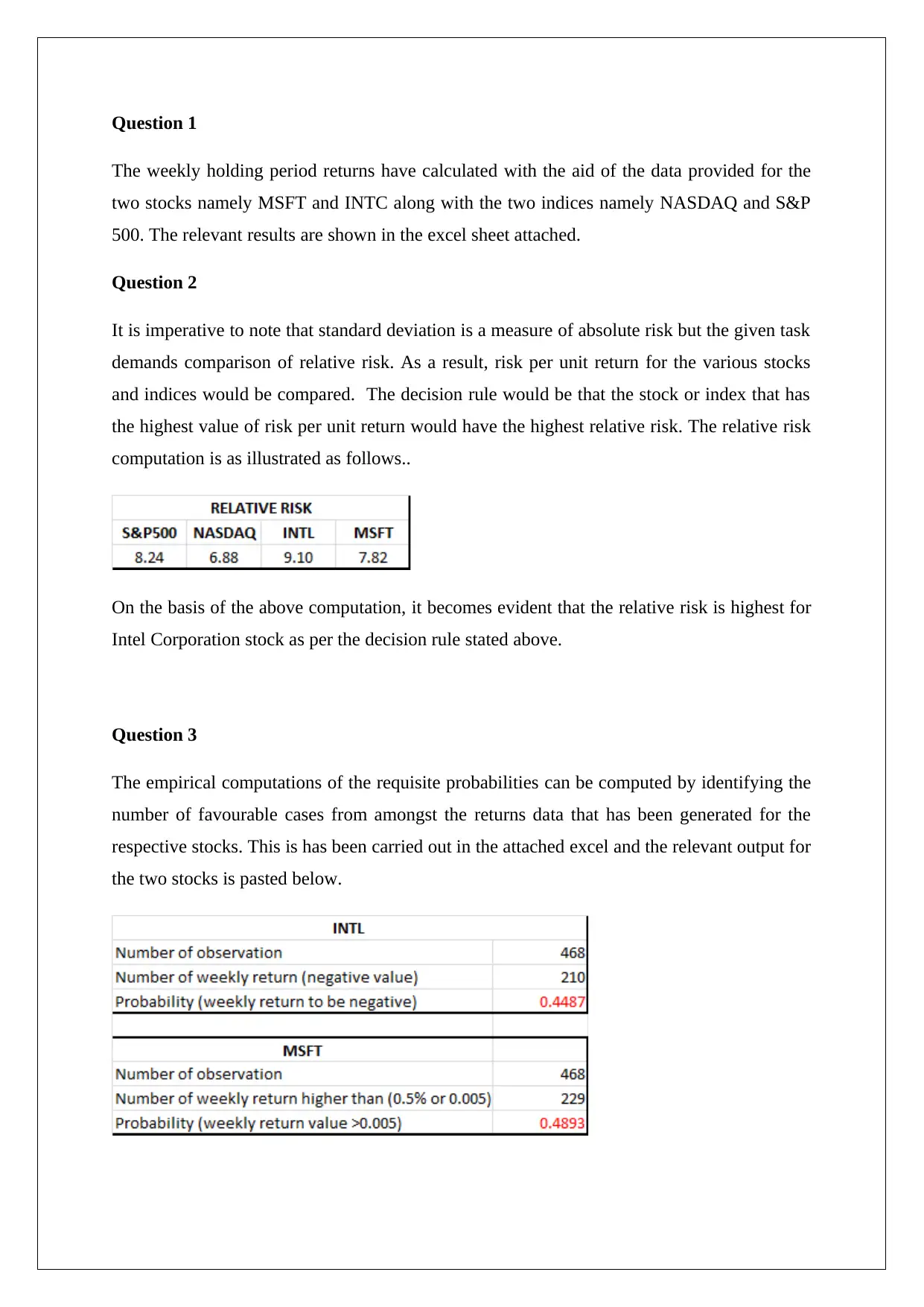
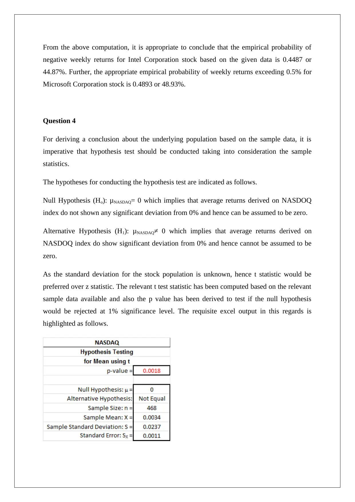
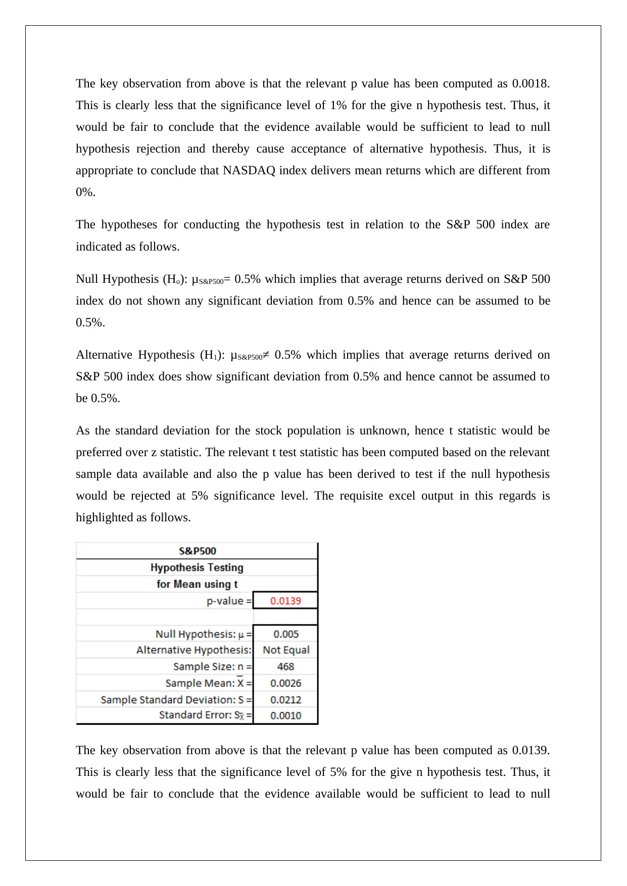
This homework assignment analyzes the performance of two stocks (MSFT and INTC) and two indices (NASDAQ and S&P 500) using provided data. The solution calculates weekly holding period returns, assesses relative risk using risk per unit return, and determines empirical probabilities of negative returns and returns exceeding a threshold. Hypothesis tests are conducted to evaluate the mean returns of NASDAQ and S&P 500. Covariance and correlation are computed for the indices and stocks, respectively. Two regression models are analyzed: Model A examines the relationship between S&P 500 and INTC returns, while Model B incorporates MSFT returns. The analysis includes assessing the significance of intercept and slope coefficients, constructing confidence intervals, and comparing the predictive power of the models based on adjusted R-squared and the coefficient of determination. The solution concludes with a preference for Model B due to its superior predictor power.

ANALYTICAL METHODS
STUDENT ID:
[Pick the date]

Question 1
The weekly holding period returns have calculated with the aid of the data provided for the
two stocks namely MSFT and INTC along with the two indices namely NASDAQ and S&P
500. The relevant results are shown in the excel sheet attached.
Question 2
It is imperative to note that standard deviation is a measure of absolute risk but the given task
demands comparison of relative risk. As a result, risk per unit return for the various stocks
and indices would be compared. The decision rule would be that the stock or index that has
the highest value of risk per unit return would have the highest relative risk. The relative risk
computation is as illustrated as follows..
On the basis of the above computation, it becomes evident that the relative risk is highest for
Intel Corporation stock as per the decision rule stated above.
Question 3
The empirical computations of the requisite probabilities can be computed by identifying the
number of favourable cases from amongst the returns data that has been generated for the
respective stocks. This is has been carried out in the attached excel and the relevant output for
the two stocks is pasted below.

From the above computation, it is appropriate to conclude that the empirical probability of
negative weekly returns for Intel Corporation stock based on the given data is 0.4487 or
44.87%. Further, the appropriate empirical probability of weekly returns exceeding 0.5% for
Microsoft Corporation stock is 0.4893 or 48.93%.
Question 4
For deriving a conclusion about the underlying population based on the sample data, it is
imperative that hypothesis test should be conducted taking into consideration the sample
statistics.
The hypotheses for conducting the hypothesis test are indicated as follows.
Null Hypothesis (Ho): μNASDAQ= 0 which implies that average returns derived on NASDOQ
index do not shown any significant deviation from 0% and hence can be assumed to be zero.
Alternative Hypothesis (H1): μNASDAQ≠ 0 which implies that average returns derived on
NASDOQ index do show significant deviation from 0% and hence cannot be assumed to be
zero.
As the standard deviation for the stock population is unknown, hence t statistic would be
preferred over z statistic. The relevant t test statistic has been computed based on the relevant
sample data available and also the p value has been derived to test if the null hypothesis
would be rejected at 1% significance level. The requisite excel output in this regards is
highlighted as follows.

The key observation from above is that the relevant p value has been computed as 0.0018.
This is clearly less that the significance level of 1% for the give n hypothesis test. Thus, it
would be fair to conclude that the evidence available would be sufficient to lead to null
hypothesis rejection and thereby cause acceptance of alternative hypothesis. Thus, it is
appropriate to conclude that NASDAQ index delivers mean returns which are different from
0%.
The hypotheses for conducting the hypothesis test in relation to the S&P 500 index are
indicated as follows.
Null Hypothesis (Ho): μS&P500= 0.5% which implies that average returns derived on S&P 500
index do not shown any significant deviation from 0.5% and hence can be assumed to be
0.5%.
Alternative Hypothesis (H1): μS&P500≠ 0.5% which implies that average returns derived on
S&P 500 index does show significant deviation from 0.5% and hence cannot be assumed to
be 0.5%.
As the standard deviation for the stock population is unknown, hence t statistic would be
preferred over z statistic. The relevant t test statistic has been computed based on the relevant
sample data available and also the p value has been derived to test if the null hypothesis
would be rejected at 5% significance level. The requisite excel output in this regards is
highlighted as follows.
The key observation from above is that the relevant p value has been computed as 0.0139.
This is clearly less that the significance level of 5% for the give n hypothesis test. Thus, it
would be fair to conclude that the evidence available would be sufficient to lead to null

hypothesis rejection and thereby cause acceptance of alternative hypothesis. Thus, it is
appropriate to conclude that S&P500 index delivers mean returns which are different from
0.5%.
Question 5
For the two indices (i.e. NASDAQ & S&P 500), covariance has been calculated using the
sample returns computed and has been derived as 0.0005. Further, for the two stocks (i.e.
MSFT & INTC), correlation has been calculated using the sample returns computed and has
been derived as 0.5557.
Question 6
The Model A regression model has been computed using S&P 500 weekly returns as the
independent variable and INTC weekly returns as the dependent variable. The output is
illustrated as follows.
6.1) Based on the above output, it needs to be determined if the intercept coefficient for the
above model is statistically significant or not. The requisite hypotheses required for testing
the hypothesis are highlighted below.
Null hypothesis: α = 0 i.e. intercept coefficient is insignificant and hence can be assumed to
be zero.

Alternative Hypothesis: α ≠ 0 i.e. intercept coefficient is significant and hence cannot be
assumed to be zero.
The regression output clearly highlights that the test statistic for the intercept coefficient is
0.86 and the p value corresponding to the above test statistic is 0.39. As this p value is not
lower than the 5% significance level, hence it would be fair to conclude that the evidence
available would be insufficient to lead to null hypothesis rejection. Thus, it would be
appropriate to conclude that for the regression model A, the intercept coefficient would not
be significant.
6.2) The objective is to estimate the 99% confidence interval for the regression slope. In this
regards, the following output is considered useful since regression is run with a confidence
interval of 99%.
The highlighted portion clearly highlights that the requisite confidence interval for the slope
would lie in the interval (0.9,1.19). Hence, we can conclude with 95% confidence that the
beta for Intel Corporation stock based on the population data would lie within the range
specified by the confidence interval.
6.3) For the regression model B, another independent variable in the form of MSFT stock
returns has been introduced and hence the given model would be a multiple regression model.
The excel output for this model is highlighted as follows.

For ascertaining if there is joint significance of the independent variables used in the model, it
is essential that ANOVA output is to be considered. The requisite hypotheses for conducting
the relevant hypothesis test are listed as follows.
Null Hypothesis (H0): The slope coefficients of both the independent variables are zero and
hence the linear model is insignificant.
Alternative Hypothesis (H1): There is atleast one independent variable which has a non-zero
slope coefficient and hence the linear model is significant.
The ANOVA result is present in the excel output for Model B. The relevant test statistic is F
whose value has been computed as 207.14. Further, the p value for the F statistic comes out
as 0. This is lesser than the level of significance of 5% for which the hypothesis test is to be
performed. Hence it would be fair to conclude that the evidence available would be
insufficient to lead to null hypothesis rejection. Thus, it would be appropriate to conclude that
for the regression model B, there is joint significance of the independent variables.
6.4) There is preference for the Model B in comparison for Model A. This is because for
Model B, both the adjusted R2 and the coefficient of determination is higher when compared
to the corresponding values for Model A. Hence, it would be appropriate to conclude that
Model B has a superior predictor power when compared to Model A. Besides, from the
output of Model B, it can also be derived that the slope coefficient for MSFT stock returns

would be considered significant at level of significance of 1% and hence it needs to be
present in the regression model for predicting the returns for INTC stock. Therefore, it may
be concluded that Model B is the better choice.