Analytical Techniques for Supply Chain Management

This document discusses various analytical techniques used in supply chain management. It includes case studies on Cranfield Grill, Supplier Selection, Record Store's Goals, and Grocery Retailer's Delivery Problem. The document covers decision variables, objective functions, constraints, and model solutions.

Analytical Techniques for Supply Chain Management
Student’s Name
Institution Affiliation
1

Case 1: Cranfield Grill
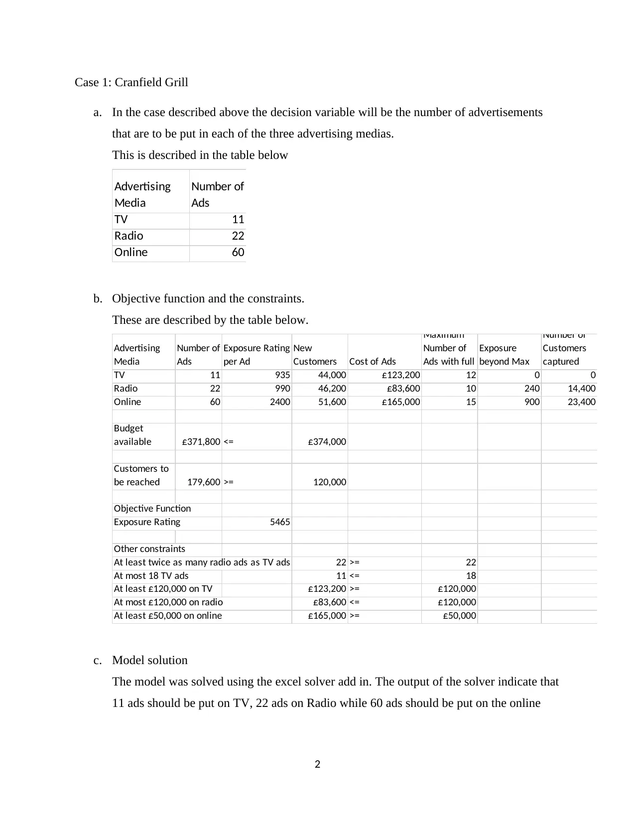
a. In the case described above the decision variable will be the number of advertisements
that are to be put in each of the three advertising medias.
This is described in the table below
Advertising
Media
Number of
Ads
TV 11
Radio 22
Online 60
b. Objective function and the constraints.
These are described by the table below.
Advertising
Media
Number of
Ads
Exposure Rating
per Ad
New
Customers Cost of Ads
Maximum
Number of
Ads with full
Exposure
beyond Max
Number of
Customers
captured
TV 11 935 44,000 £123,200 12 0 0
Radio 22 990 46,200 £83,600 10 240 14,400
Online 60 2400 51,600 £165,000 15 900 23,400
Budget
available £371,800 <= £374,000
Customers to
be reached 179,600 >= 120,000
Objective Function
Exposure Rating 5465
Other constraints
At least twice as many radio ads as TV ads 22 >= 22
At most 18 TV ads 11 <= 18
At least £120,000 on TV £123,200 >= £120,000
At most £120,000 on radio £83,600 <= £120,000
At least £50,000 on online £165,000 >= £50,000
c. Model solution
The model was solved using the excel solver add in. The output of the solver indicate that
11 ads should be put on TV, 22 ads on Radio while 60 ads should be put on the online
2

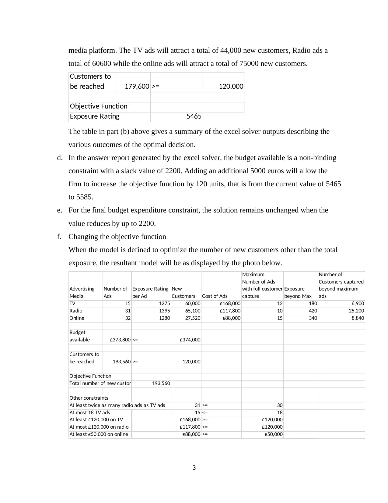
media platform. The TV ads will attract a total of 44,000 new customers, Radio ads a
total of 60600 while the online ads will attract a total of 75000 new customers.
Customers to
be reached 179,600 >= 120,000
Objective Function
Exposure Rating 5465
The table in part (b) above gives a summary of the excel solver outputs describing the
various outcomes of the optimal decision.
d. In the answer report generated by the excel solver, the budget available is a non-binding
constraint with a slack value of 2200. Adding an additional 5000 euros will allow the
firm to increase the objective function by 120 units, that is from the current value of 5465
to 5585.
e. For the final budget expenditure constraint, the solution remains unchanged when the
value reduces by up to 2200.
f. Changing the objective function
When the model is defined to optimize the number of new customers other than the total
exposure, the resultant model will be as displayed by the photo below.
Advertising
Media
Number of
Ads
Exposure Rating
per Ad
New
Customers Cost of Ads
Maximum
Number of Ads
with full customer
capture
Exposure
beyond Max
Number of
Customers captured
beyond maximum
ads
TV 15 1275 60,000 £168,000 12 180 6,900
Radio 31 1395 65,100 £117,800 10 420 25,200
Online 32 1280 27,520 £88,000 15 340 8,840
Budget
available £373,800 <= £374,000
Customers to
be reached 193,560 >= 120,000
Objective Function
Total number of new customers 193,560
Other constraints
At least twice as many radio ads as TV ads 31 >= 30
At most 18 TV ads 15 <= 18
At least £120,000 on TV £168,000 >= £120,000
At most £120,000 on radio £117,800 <= £120,000
At least £50,000 on online £88,000 >= £50,000
3

From the table the total budget utilized will be 373,800 which is higher than the 371800
which was utilized previously. In addition, the total new customers acquired will go up
from 179,600 to 193,560.
g. Best objective function.
The best objective function is the total number of new customers acquired. The aim of
advertising a restaurant is to increase its sales revenue. This is optimized when the
number of new customers acquired goes up. Since maximizing the total number of
customers optimizes the number of new customers acquired more than maximizing the
total exposure, it is the most preferred objective function (Lewis, 2009).
Case 2: Supplier Selection
a. Weight of the main criteria
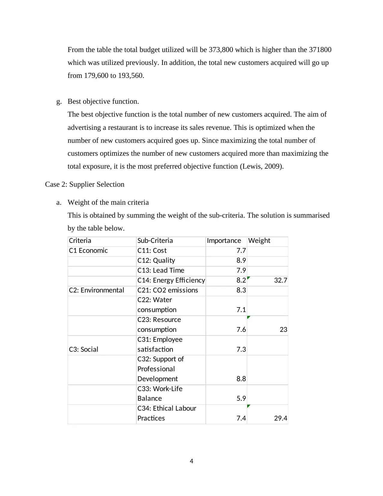
This is obtained by summing the weight of the sub-criteria. The solution is summarised
by the table below.
Criteria Sub-Criteria Importance Weight
C1 Economic C11: Cost 7.7
C12: Quality 8.9
C13: Lead Time 7.9
C14: Energy Efficiency 8.2 32.7
C2: Environmental C21: CO2 emissions 8.3
C22: Water
consumption 7.1
C23: Resource
consumption 7.6 23
C3: Social
C31: Employee
satisfaction 7.3
C32: Support of
Professional
Development 8.8
C33: Work-Life
Balance 5.9
C34: Ethical Labour
Practices 7.4 29.4
4

b. Using the AHP system, the criteria are ranked based in the best possible impact socially,
economically and environmentally. This generates a consistence result as the product
demanded will be able to ensure sustainability.
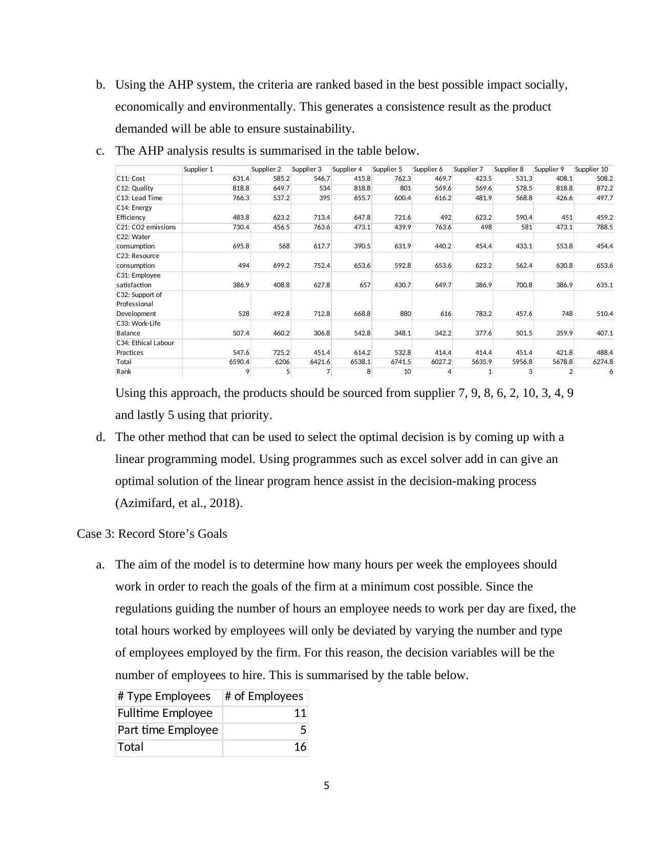
c. The AHP analysis results is summarised in the table below.
Supplier 1 Supplier 2 Supplier 3 Supplier 4 Supplier 5 Supplier 6 Supplier 7 Supplier 8 Supplier 9 Supplier 10
C11: Cost 631.4 585.2 546.7 415.8 762.3 469.7 423.5 531.3 408.1 508.2
C12: Quality 818.8 649.7 534 818.8 801 569.6 569.6 578.5 818.8 872.2
C13: Lead Time 766.3 537.2 395 655.7 600.4 616.2 481.9 568.8 426.6 497.7
C14: Energy
Efficiency 483.8 623.2 713.4 647.8 721.6 492 623.2 590.4 451 459.2
C21: CO2 emissions 730.4 456.5 763.6 473.1 439.9 763.6 498 581 473.1 788.5
C22: Water
consumption 695.8 568 617.7 390.5 631.9 440.2 454.4 433.1 553.8 454.4
C23: Resource
consumption 494 699.2 752.4 653.6 592.8 653.6 623.2 562.4 630.8 653.6
C31: Employee
satisfaction 386.9 408.8 627.8 657 430.7 649.7 386.9 700.8 386.9 635.1
C32: Support of
Professional
Development 528 492.8 712.8 668.8 880 616 783.2 457.6 748 510.4
C33: Work-Life
Balance 507.4 460.2 306.8 542.8 348.1 342.2 377.6 501.5 359.9 407.1
C34: Ethical Labour
Practices 547.6 725.2 451.4 614.2 532.8 414.4 414.4 451.4 421.8 488.4
Total 6590.4 6206 6421.6 6538.1 6741.5 6027.2 5635.9 5956.8 5678.8 6274.8
Rank 9 5 7 8 10 4 1 3 2 6
Using this approach, the products should be sourced from supplier 7, 9, 8, 6, 2, 10, 3, 4, 9
and lastly 5 using that priority.
d. The other method that can be used to select the optimal decision is by coming up with a
linear programming model. Using programmes such as excel solver add in can give an
optimal solution of the linear program hence assist in the decision-making process
(Azimifard, et al., 2018).
Case 3: Record Store’s Goals
a. The aim of the model is to determine how many hours per week the employees should
work in order to reach the goals of the firm at a minimum cost possible. Since the
regulations guiding the number of hours an employee needs to work per day are fixed, the
total hours worked by employees will only be deviated by varying the number and type
of employees employed by the firm. For this reason, the decision variables will be the
number of employees to hire. This is summarised by the table below.
# Type Employees # of Employees
Fulltime Employee 11
Part time Employee 5
Total 16
5

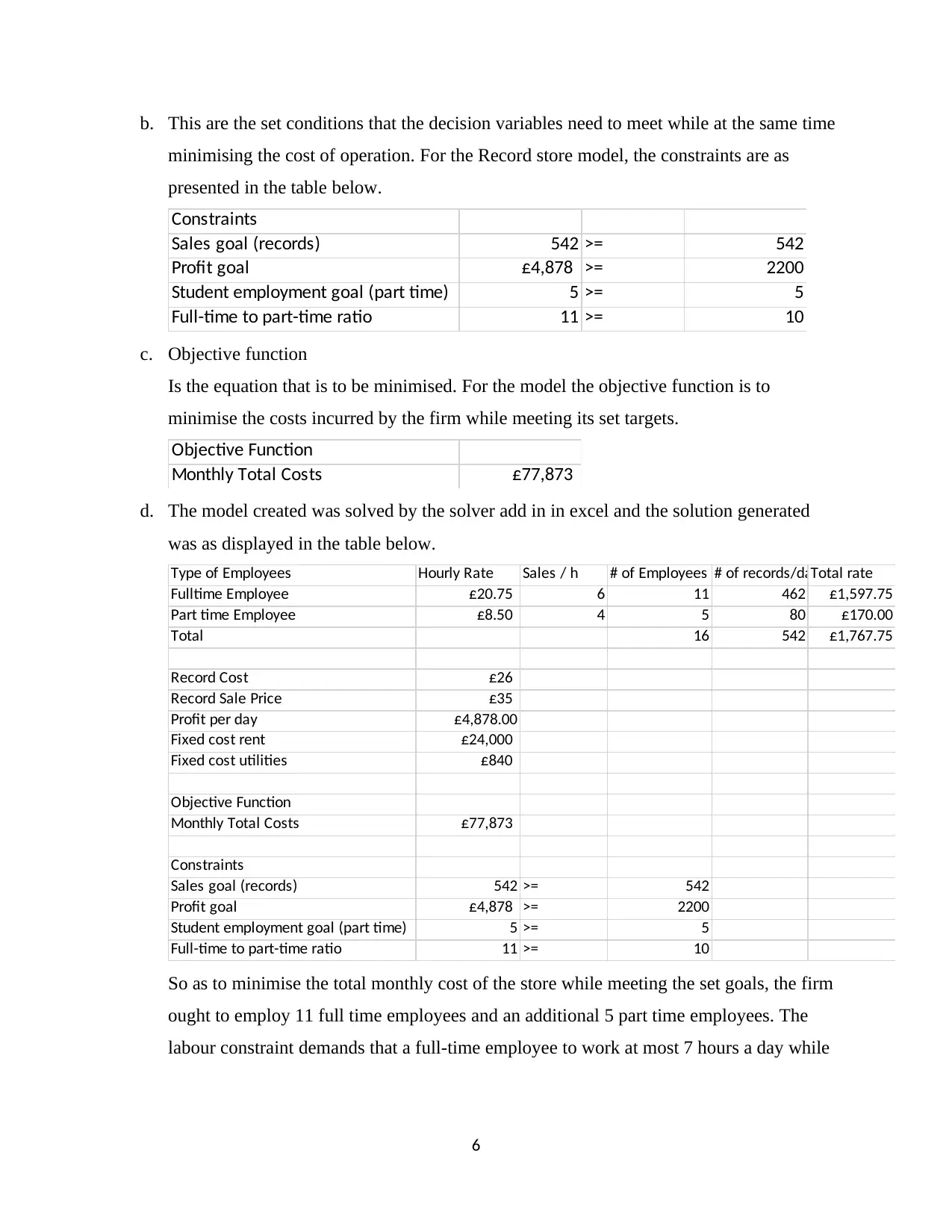
b. This are the set conditions that the decision variables need to meet while at the same time
minimising the cost of operation. For the Record store model, the constraints are as
presented in the table below.
Constraints
Sales goal (records) 542 >= 542
Profit goal £4,878 >= 2200
Student employment goal (part time) 5 >= 5
Full-time to part-time ratio 11 >= 10
c. Objective function
Is the equation that is to be minimised. For the model the objective function is to
minimise the costs incurred by the firm while meeting its set targets.
Objective Function
Monthly Total Costs £77,873
d. The model created was solved by the solver add in in excel and the solution generated
was as displayed in the table below.
Type of Employees Hourly Rate Sales / h # of Employees # of records/dayTotal rate
Fulltime Employee £20.75 6 11 462 £1,597.75
Part time Employee £8.50 4 5 80 £170.00
Total 16 542 £1,767.75
Record Cost £26
Record Sale Price £35
Profit per day £4,878.00
Fixed cost rent £24,000
Fixed cost utilities £840
Objective Function
Monthly Total Costs £77,873
Constraints
Sales goal (records) 542 >= 542
Profit goal £4,878 >= 2200
Student employment goal (part time) 5 >= 5
Full-time to part-time ratio 11 >= 10
So as to minimise the total monthly cost of the store while meeting the set goals, the firm
ought to employ 11 full time employees and an additional 5 part time employees. The
labour constraint demands that a full-time employee to work at most 7 hours a day while
6

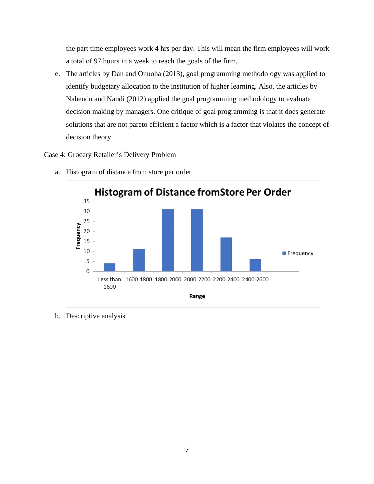
the part time employees work 4 hrs per day. This will mean the firm employees will work
a total of 97 hours in a week to reach the goals of the firm.
e. The articles by Dan and Onuoha (2013), goal programming methodology was applied to
identify budgetary allocation to the institution of higher learning. Also, the articles by
Nabendu and Nandi (2012) applied the goal programming methodology to evaluate
decision making by managers. One critique of goal programming is that it does generate
solutions that are not pareto efficient a factor which is a factor that violates the concept of
decision theory.
Case 4: Grocery Retailer’s Delivery Problem
a. Histogram of distance from store per order
b. Descriptive analysis
7

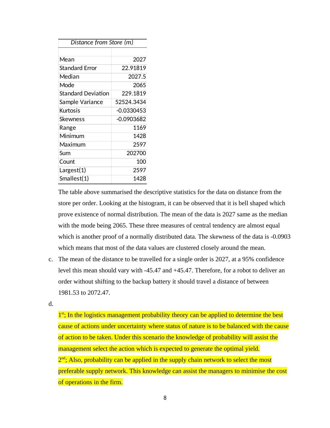
Distance from Store (m)
Mean 2027
Standard Error 22.91819
Median 2027.5
Mode 2065
Standard Deviation 229.1819
Sample Variance 52524.3434
Kurtosis -0.0330453
Skewness -0.0903682
Range 1169
Minimum 1428
Maximum 2597
Sum 202700
Count 100
Largest(1) 2597
Smallest(1) 1428
The table above summarised the descriptive statistics for the data on distance from the
store per order. Looking at the histogram, it can be observed that it is bell shaped which
prove existence of normal distribution. The mean of the data is 2027 same as the median
with the mode being 2065. These three measures of central tendency are almost equal
which is another proof of a normally distributed data. The skewness of the data is -0.0903
which means that most of the data values are clustered closely around the mean.
c. The mean of the distance to be travelled for a single order is 2027, at a 95% confidence
level this mean should vary with -45.47 and +45.47. Therefore, for a robot to deliver an
order without shifting to the backup battery it should travel a distance of between
1981.53 to 2072.47.
d.
1st; In the logistics management probability theory can be applied to determine the best
cause of actions under uncertainty where status of nature is to be balanced with the cause
of action to be taken. Under this scenario the knowledge of probability will assist the
management select the action which is expected to generate the optimal yield.
2nd; Also, probability can be applied in the supply chain network to select the most
preferable supply network. This knowledge can assist the managers to minimise the cost
of operations in the firm.
8

3rd; Finally, probability theory can be applied in modelling the future sales volume, this is
crucial especially in designing the production system to meet the future demand at the
minimal cost possible (Grinstead & Snell, n.d.).
Case 5: A Fashion Retailer’s Sales Forecast
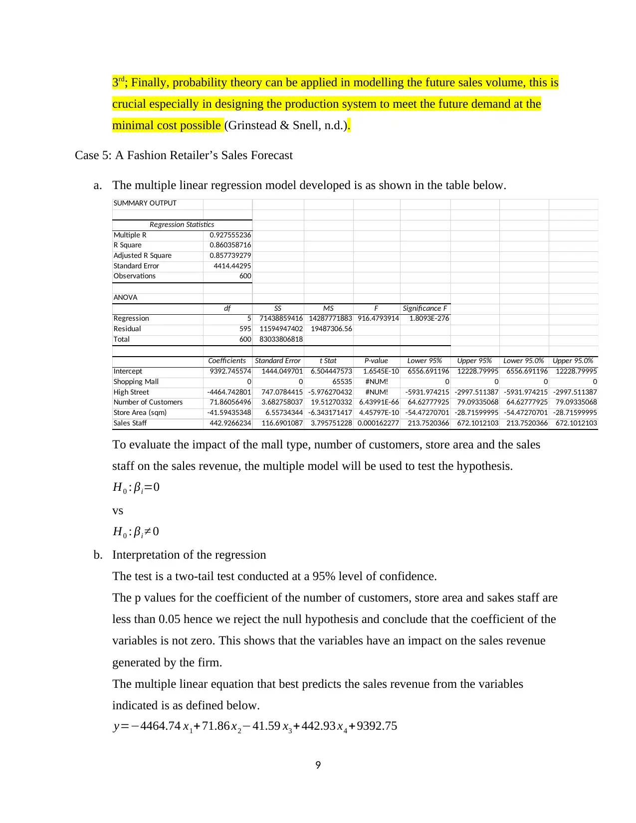
a. The multiple linear regression model developed is as shown in the table below.
SUMMARY OUTPUT
Regression Statistics
Multiple R 0.927555236
R Square 0.860358716
Adjusted R Square 0.857739279
Standard Error 4414.44295
Observations 600
ANOVA
df SS MS F Significance F
Regression 5 71438859416 14287771883 916.4793914 1.8093E-276
Residual 595 11594947402 19487306.56
Total 600 83033806818
Coefficients Standard Error t Stat P-value Lower 95% Upper 95% Lower 95.0% Upper 95.0%
Intercept 9392.745574 1444.049701 6.504447573 1.6545E-10 6556.691196 12228.79995 6556.691196 12228.79995
Shopping Mall 0 0 65535 #NUM! 0 0 0 0
High Street -4464.742801 747.0784415 -5.976270432 #NUM! -5931.974215 -2997.511387 -5931.974215 -2997.511387
Number of Customers 71.86056496 3.682758037 19.51270332 6.43991E-66 64.62777925 79.09335068 64.62777925 79.09335068
Store Area (sqm) -41.59435348 6.55734344 -6.343171417 4.45797E-10 -54.47270701 -28.71599995 -54.47270701 -28.71599995
Sales Staff 442.9266234 116.6901087 3.795751228 0.000162277 213.7520366 672.1012103 213.7520366 672.1012103
To evaluate the impact of the mall type, number of customers, store area and the sales
staff on the sales revenue, the multiple model will be used to test the hypothesis.
H0 : βi=0
vs
H0 : βi ≠ 0
b. Interpretation of the regression
The test is a two-tail test conducted at a 95% level of confidence.
The p values for the coefficient of the number of customers, store area and sakes staff are
less than 0.05 hence we reject the null hypothesis and conclude that the coefficient of the
variables is not zero. This shows that the variables have an impact on the sales revenue
generated by the firm.
The multiple linear equation that best predicts the sales revenue from the variables
indicated is as defined below.
y=−4464.74 x1+ 71.86 x2−41.59 x3 + 442.93 x4 +9392.75
9

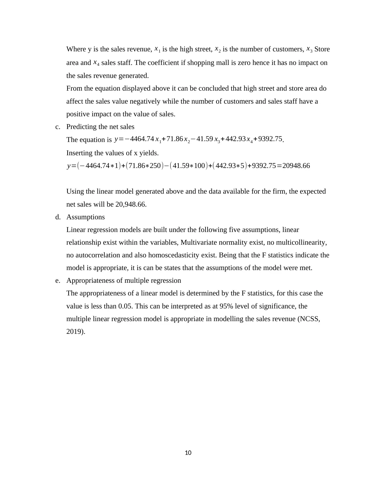
Where y is the sales revenue, x1 is the high street, x2 is the number of customers, x3 Store
area and x4 sales staff. The coefficient if shopping mall is zero hence it has no impact on
the sales revenue generated.
From the equation displayed above it can be concluded that high street and store area do
affect the sales value negatively while the number of customers and sales staff have a
positive impact on the value of sales.
c. Predicting the net sales
The equation is y=−4464.74 x1+71.86 x2−41.59 x3 +442.93 x4 + 9392.75.
Inserting the values of x yields.
y=(−4464.74∗1)+(71.86∗250)−( 41.59∗100)+( 442.93∗5)+9392.75=20948.66
Using the linear model generated above and the data available for the firm, the expected
net sales will be 20,948.66.
d. Assumptions
Linear regression models are built under the following five assumptions, linear
relationship exist within the variables, Multivariate normality exist, no multicollinearity,
no autocorrelation and also homoscedasticity exist. Being that the F statistics indicate the
model is appropriate, it is can be states that the assumptions of the model were met.
e. Appropriateness of multiple regression
The appropriateness of a linear model is determined by the F statistics, for this case the
value is less than 0.05. This can be interpreted as at 95% level of significance, the
multiple linear regression model is appropriate in modelling the sales revenue (NCSS,
2019).
10

References
Azimifard, A., Moosavirad, S. H. & Ariafar, S., 2018. Selecting sustainable supplier countries for Iran's
steel industry at three levels by using AHP and TOPSIS methods. Resources Policy, Volume 57,
pp. 30-44.
Dan, D. E. & Onuoha, D. O., 2013. GOAL PROGRAMMING: - AN APPLICATION TO
BUDGETARY ALLOCATION OF AN INSTITUTION OF HIGHER LEARNING. Research
Journal in Engineering and Applied Sciences , 2(2), pp. 95-105 .
Grinstead, C. M. & Snell, J. L., n.d. Introduction to Probability. [Online]
Available at:
https://www.dartmouth.edu/~chance/teaching_aids/books_articles/probability_book/
amsbook.mac.pdf
[Accessed 25 May 2019].
Lewis, C., 2009. Linear Programming: Theory and Applications. [Online]
Available at: https://www.whitman.edu/Documents/Academics/Mathematics/lewis.pdf
[Accessed 27 May 2019].
Nabendu, S. & Nandi, M., 2012. Goal Programming, its Application in Management Sectors– Special
Attention into Plantation Management. International Journal of Scientific and Research
Publications, 2(9).
NCSS, 2019. Linear Regression and Correlation. [Online]
Available at: https://ncss-wpengine.netdna-ssl.com/wp-content/themes/ncss/pdf/Procedures/
NCSS/Linear_Regression_and_Correlation.pdf
[Accessed 25 May 2019].
11