Significant Interaction Effects in Studies

This assignment involves analyzing two separate studies that examine the impact of different factors on individuals' responses. The first study investigates the relationship between disgust levels and fear scores, providing evidence to support the researchers' hypothesis. The second study assesses the interaction effect of time of measurement and swearing group on positive attitudes towards a topic, revealing significant differences and implications for further research.

Running Head: QUANTITATIVE ASSIGNMENT
Quantitative Assignment
Name of the Student
Name of the University
Author Note

QUANTITATIVE ASSIGNMENT1
Table of Contents
Part A...............................................................................................................................................2
Answer 1......................................................................................................................................2
Answer 2......................................................................................................................................4
Answer 3......................................................................................................................................4
Answer 4......................................................................................................................................5
Answer 5......................................................................................................................................6
Part B...............................................................................................................................................7

QUANTITATIVE ASSIGNMENT2
Part A
People fear for different types of animals and insects. The fear for spiders, rats and
snakes are more common than fear from rabbits or giraffes. According to a study conducted by
Davey (1994), the fear for small animals such as spiders come from disgust. Thus, he
hypothesized that people with higher disgust propensity are more likely to be feared than the
ones with lower disgust propensity. This study has been conducted to investigate the proposal
stated by Davey. The study was conducted on 150 participants. All the participants filled in a
questionnaire to measure their level of fear from spider.
Answer 1
In order to determine the outliers to the data, the upper and the lower bound of the
outliers have to be evaluated. The upper and the lower outlier ranges are given by the formula:
Upper Outlier Range: Third Quartile + 1.5 * Interquartile Range = 28.09 + 1.5 * 20.84 = 59.35
Lower Outlier Range: First Quartile – 1.5 * Interquartile Range = 7.25 – 1.5 * 20.84 = – 24.01
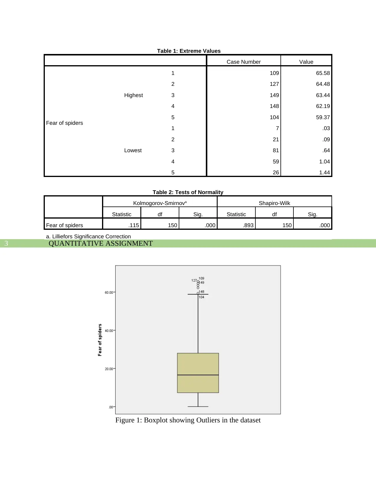
The Extreme values as given in the following table 1 shows that there are no values in the dataset
lower than – 24.01 but there are 5 values higher than 59.35. Thus, there are 5 outliers to the
dataset. The outliers are also shown diagrammatically in figure 1.
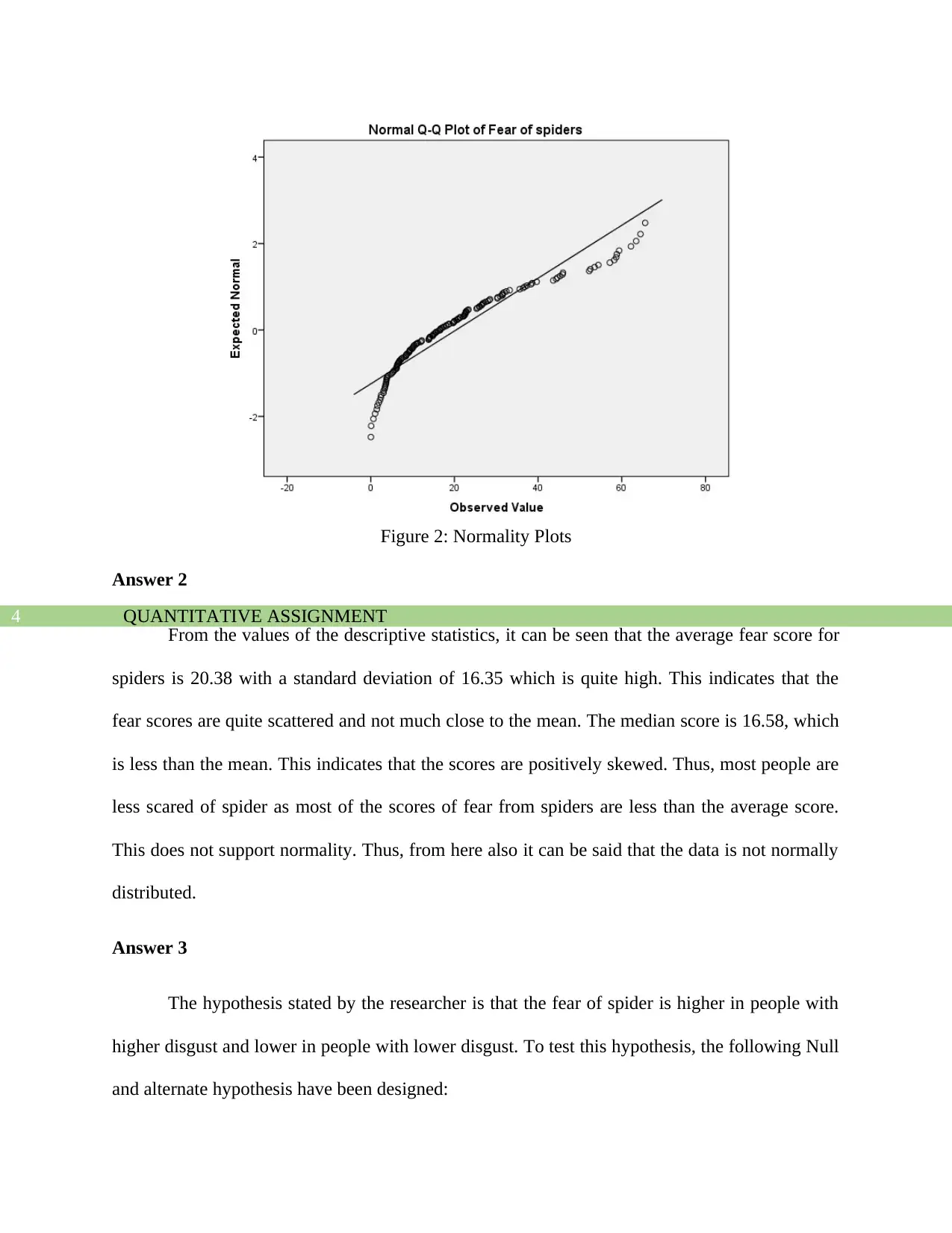
It can be seen from table 2 that the normality statistic has been obtained as 0.115, which
is higher than the critical value of the normality statistic obtained from the table for 150 degrees
of freedom at 95% level of significance. Thus, it can be said the data is not normal. Figure 2 also
shows that the residuals of the data are not linear. Thus, it can be said that the data is not normal.

QUANTITATIVE ASSIGNMENT3
Table 1: Extreme Values
Case Number Value
Fear of spiders
Highest
1 109 65.58
2 127 64.48
3 149 63.44
4 148 62.19
5 104 59.37
Lowest
1 7 .03
2 21 .09
3 81 .64
4 59 1.04
5 26 1.44
Table 2: Tests of Normality
Kolmogorov-Smirnova Shapiro-Wilk
Statistic df Sig. Statistic df Sig.
Fear of spiders .115 150 .000 .893 150 .000
a. Lilliefors Significance Correction
Figure 1: Boxplot showing Outliers in the dataset

QUANTITATIVE ASSIGNMENT4
Figure 2: Normality Plots
Answer 2
From the values of the descriptive statistics, it can be seen that the average fear score for
spiders is 20.38 with a standard deviation of 16.35 which is quite high. This indicates that the
fear scores are quite scattered and not much close to the mean. The median score is 16.58, which
is less than the mean. This indicates that the scores are positively skewed. Thus, most people are
less scared of spider as most of the scores of fear from spiders are less than the average score.
This does not support normality. Thus, from here also it can be said that the data is not normally
distributed.
Answer 3
The hypothesis stated by the researcher is that the fear of spider is higher in people with
higher disgust and lower in people with lower disgust. To test this hypothesis, the following Null
and alternate hypothesis have been designed:

QUANTITATIVE ASSIGNMENT5
Null Hypothesis (H0): The fear of spider does not differ between people with different levels of
disgust.
Alternate Hypothesis (HA): The fear of spider differs between people with different levels of
disgust.
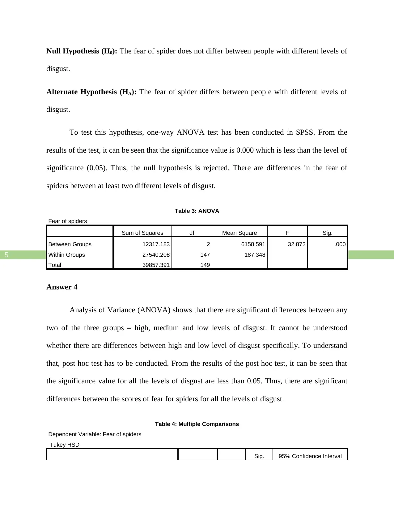
To test this hypothesis, one-way ANOVA test has been conducted in SPSS. From the
results of the test, it can be seen that the significance value is 0.000 which is less than the level of
significance (0.05). Thus, the null hypothesis is rejected. There are differences in the fear of
spiders between at least two different levels of disgust.
Table 3: ANOVA
Fear of spiders
Sum of Squares df Mean Square F Sig.
Between Groups 12317.183 2 6158.591 32.872 .000
Within Groups 27540.208 147 187.348
Total 39857.391 149
Answer 4
Analysis of Variance (ANOVA) shows that there are significant differences between any
two of the three groups – high, medium and low levels of disgust. It cannot be understood
whether there are differences between high and low level of disgust specifically. To understand
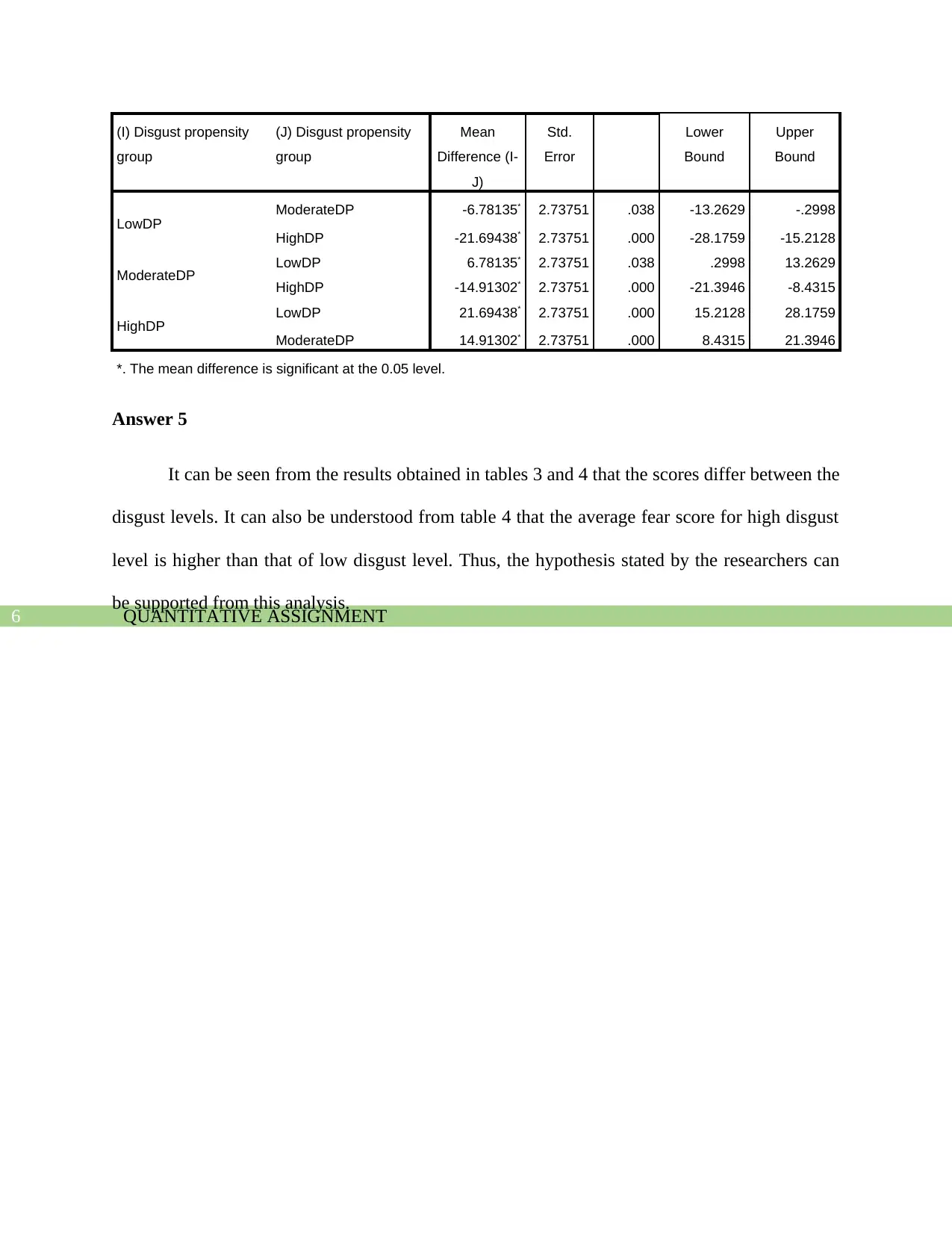
that, post hoc test has to be conducted. From the results of the post hoc test, it can be seen that
the significance value for all the levels of disgust are less than 0.05. Thus, there are significant
differences between the scores of fear for spiders for all the levels of disgust.
Table 4: Multiple Comparisons
Dependent Variable: Fear of spiders
Tukey HSD
Sig. 95% Confidence Interval

QUANTITATIVE ASSIGNMENT6
(I) Disgust propensity
group
(J) Disgust propensity
group
Mean
Difference (I-
J)
Std.
Error
Lower
Bound
Upper
Bound
LowDP ModerateDP -6.78135* 2.73751 .038 -13.2629 -.2998
HighDP -21.69438* 2.73751 .000 -28.1759 -15.2128
ModerateDP LowDP 6.78135* 2.73751 .038 .2998 13.2629
HighDP -14.91302* 2.73751 .000 -21.3946 -8.4315
HighDP LowDP 21.69438* 2.73751 .000 15.2128 28.1759
ModerateDP 14.91302* 2.73751 .000 8.4315 21.3946
*. The mean difference is significant at the 0.05 level.
Answer 5
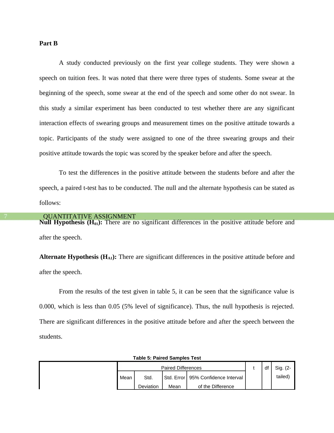
It can be seen from the results obtained in tables 3 and 4 that the scores differ between the
disgust levels. It can also be understood from table 4 that the average fear score for high disgust
level is higher than that of low disgust level. Thus, the hypothesis stated by the researchers can
be supported from this analysis.

QUANTITATIVE ASSIGNMENT7
Part B
A study conducted previously on the first year college students. They were shown a
speech on tuition fees. It was noted that there were three types of students. Some swear at the
beginning of the speech, some swear at the end of the speech and some other do not swear. In
this study a similar experiment has been conducted to test whether there are any significant
interaction effects of swearing groups and measurement times on the positive attitude towards a
topic. Participants of the study were assigned to one of the three swearing groups and their
positive attitude towards the topic was scored by the speaker before and after the speech.
To test the differences in the positive attitude between the students before and after the
speech, a paired t-test has to be conducted. The null and the alternate hypothesis can be stated as
follows:
Null Hypothesis (H01): There are no significant differences in the positive attitude before and
after the speech.
Alternate Hypothesis (HA1): There are significant differences in the positive attitude before and
after the speech.
From the results of the test given in table 5, it can be seen that the significance value is
0.000, which is less than 0.05 (5% level of significance). Thus, the null hypothesis is rejected.
There are significant differences in the positive attitude before and after the speech between the
students.
Table 5: Paired Samples Test
Paired Differences t df Sig. (2-
tailed)Mean Std.
Deviation
Std. Error
Mean
95% Confidence Interval
of the Difference

QUANTITATIVE ASSIGNMENT8
Lower Upper
Pair
1
Positive attitude before
speech - Positive attitude
after speech
-
73.54 68.376 7.895 -89.270 -57.806 -
9.314 74 .000
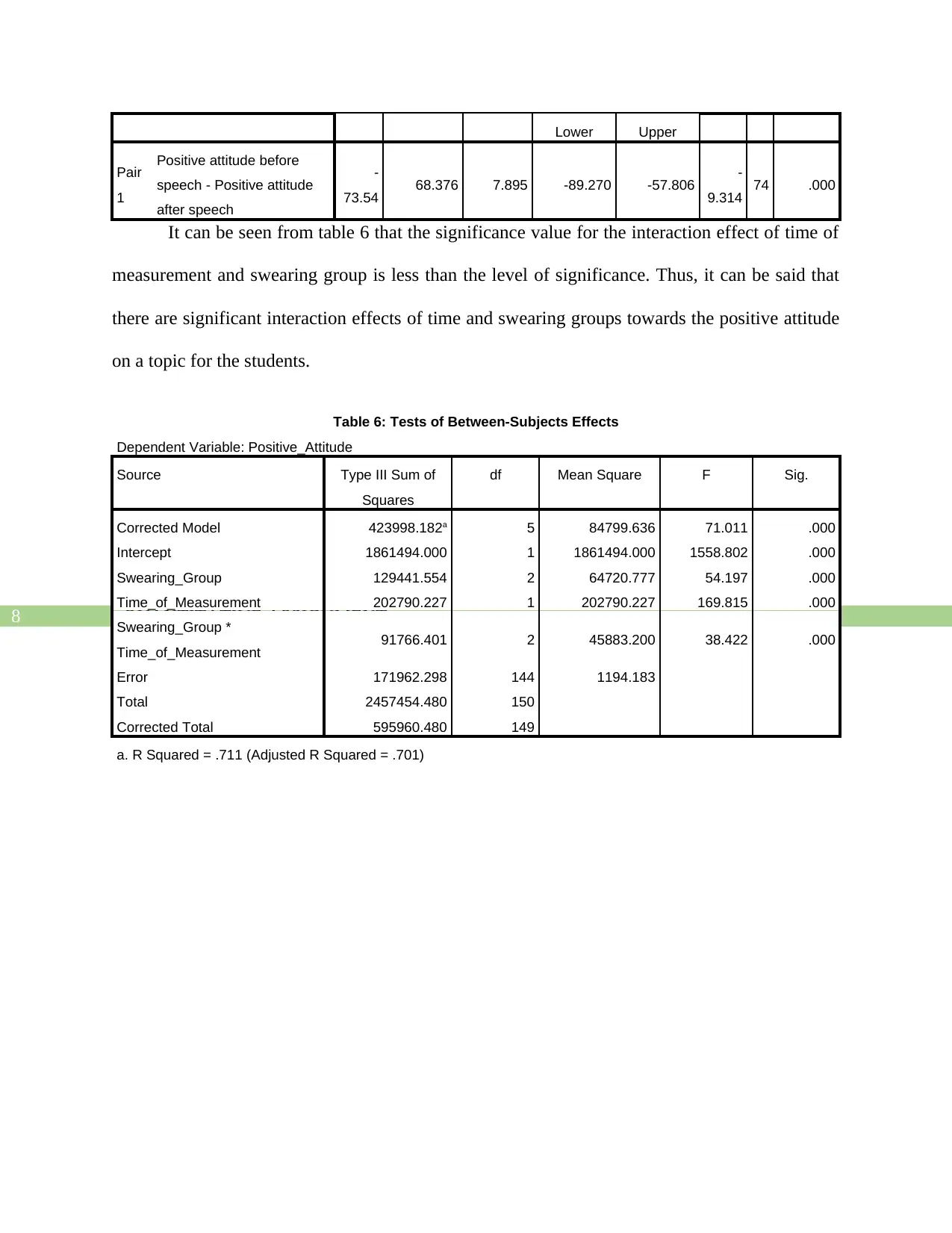
It can be seen from table 6 that the significance value for the interaction effect of time of
measurement and swearing group is less than the level of significance. Thus, it can be said that
there are significant interaction effects of time and swearing groups towards the positive attitude
on a topic for the students.
Table 6: Tests of Between-Subjects Effects
Dependent Variable: Positive_Attitude
Source Type III Sum of
Squares
df Mean Square F Sig.
Corrected Model 423998.182a 5 84799.636 71.011 .000
Intercept 1861494.000 1 1861494.000 1558.802 .000
Swearing_Group 129441.554 2 64720.777 54.197 .000
Time_of_Measurement 202790.227 1 202790.227 169.815 .000
Swearing_Group *
Time_of_Measurement 91766.401 2 45883.200 38.422 .000
Error 171962.298 144 1194.183
Total 2457454.480 150
Corrected Total 595960.480 149
a. R Squared = .711 (Adjusted R Squared = .701)