Comprehensive Solution: ANOVA, Regression Analysis Homework

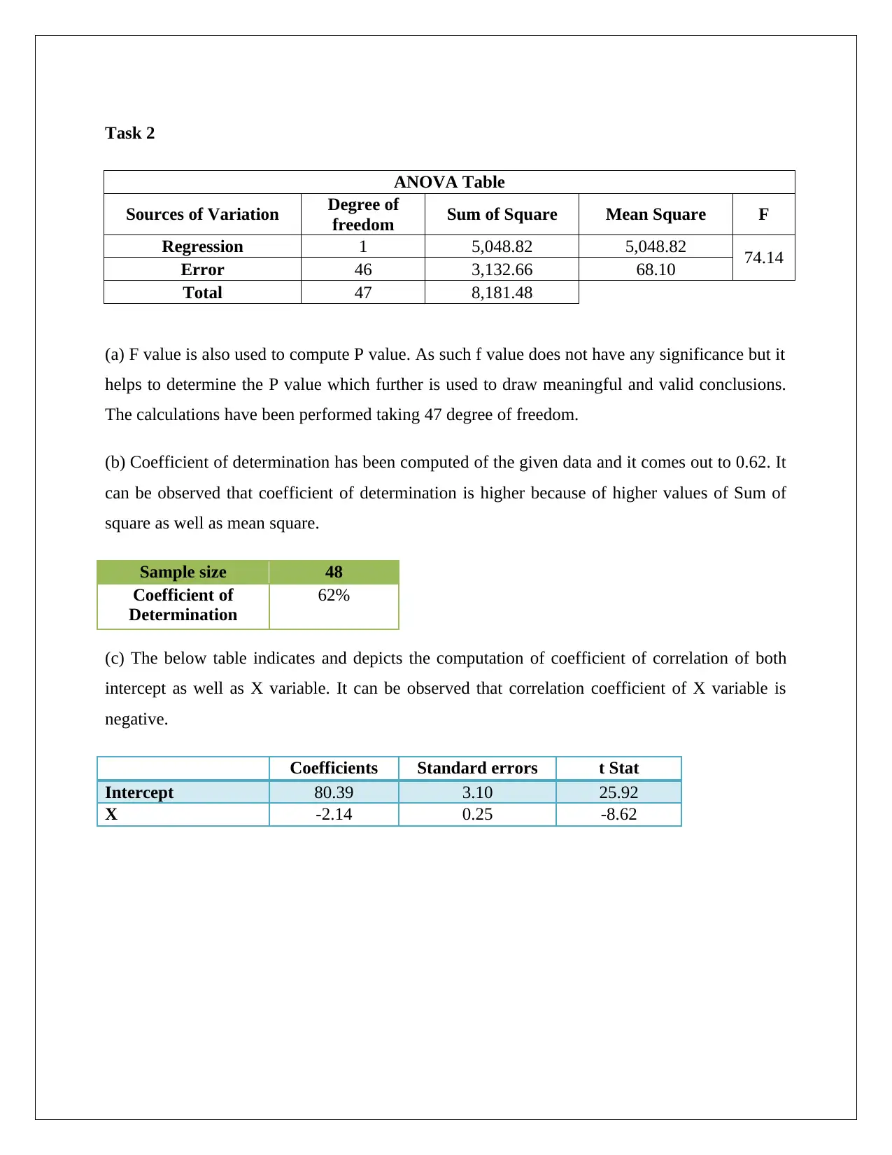
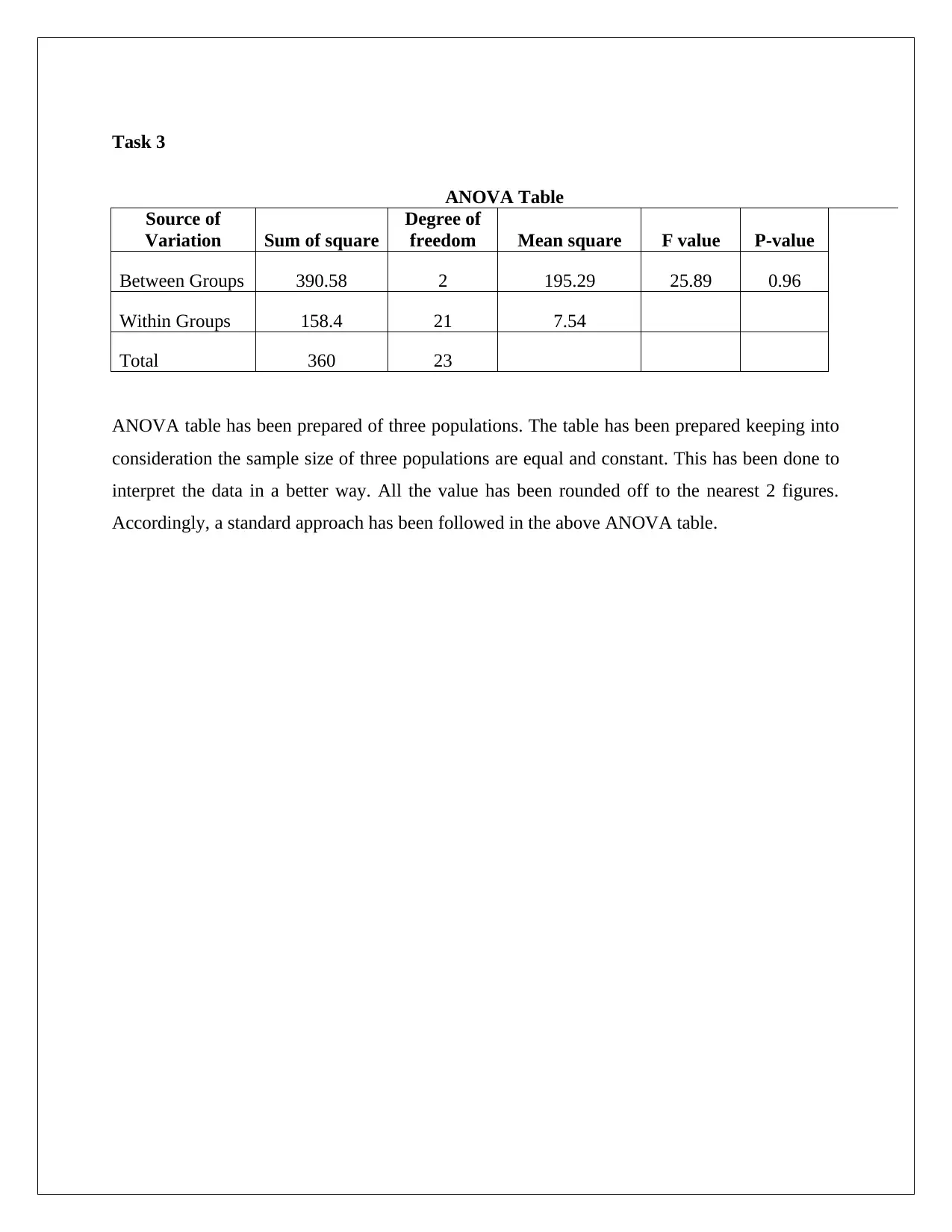
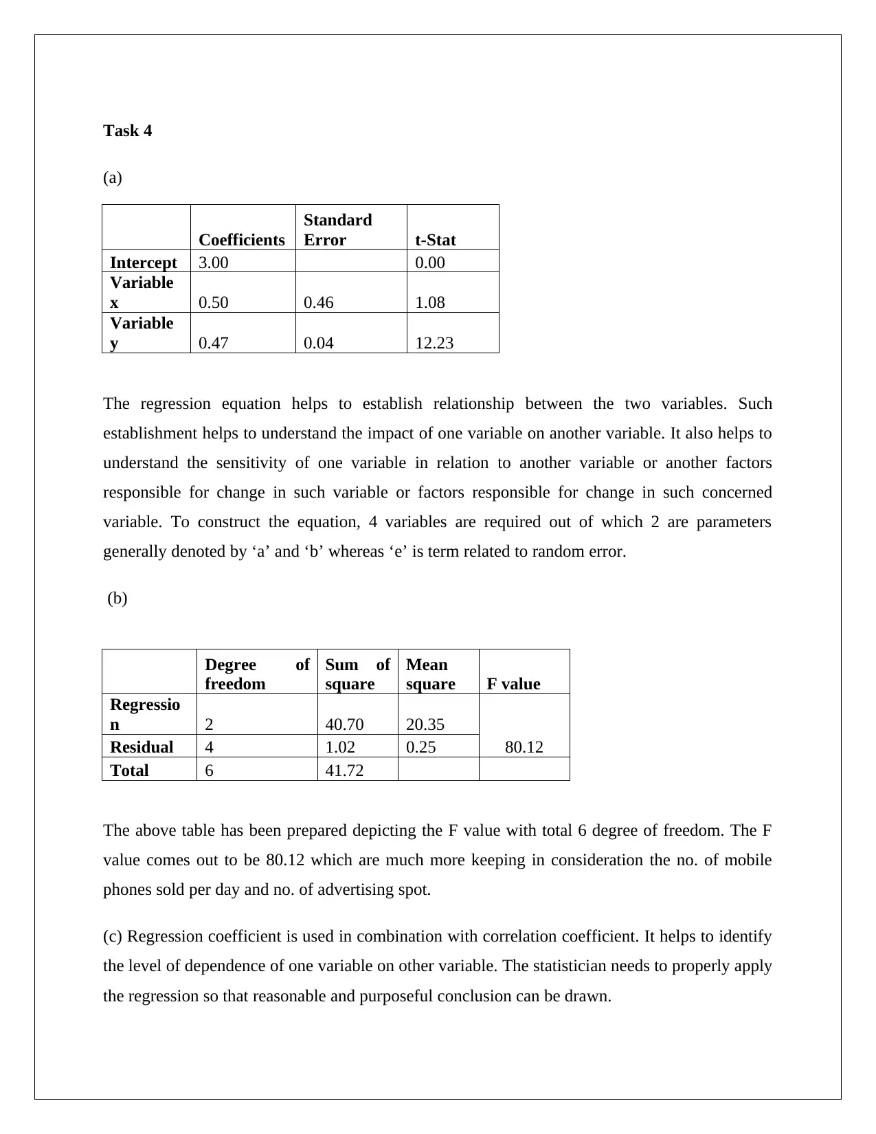
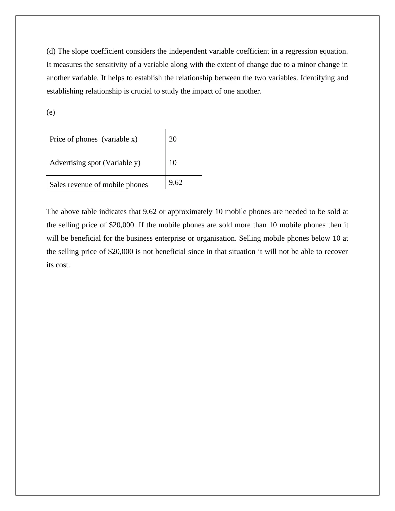
This assignment solution focuses on ANOVA and regression analysis, covering topics such as F-value interpretation, coefficient of determination, and regression coefficients. It includes calculations and interpretations related to ANOVA tables, regression equations, and the relationship between variables. Specifically, it addresses tasks involving the computation and analysis of variance, correlation coefficients, and the impact of variables on sales revenue. The solution provides detailed explanations and calculations to help understand the underlying statistical concepts and their practical applications in business scenarios. Desklib offers a wide range of similar solved assignments and study resources for students.

Task 2
ANOVA Table
Sources of Variation Degree of
freedom Sum of Square Mean Square F
Regression 1 5,048.82 5,048.82 74.14
Error 46 3,132.66 68.10
Total 47 8,181.48
(a) F value is also used to compute P value. As such f value does not have any significance but it
helps to determine the P value which further is used to draw meaningful and valid conclusions.
The calculations have been performed taking 47 degree of freedom.
(b) Coefficient of determination has been computed of the given data and it comes out to 0.62. It
can be observed that coefficient of determination is higher because of higher values of Sum of
square as well as mean square.
Sample size 48
Coefficient of
Determination
62%
(c) The below table indicates and depicts the computation of coefficient of correlation of both
intercept as well as X variable. It can be observed that correlation coefficient of X variable is
negative.
Coefficients Standard errors t Stat
Intercept 80.39 3.10 25.92
X -2.14 0.25 -8.62

Task 3
ANOVA Table
Source of
Variation Sum of square
Degree of
freedom Mean square F value P-value
Between Groups 390.58 2 195.29 25.89 0.96
Within Groups 158.4 21 7.54
Total 360 23
ANOVA table has been prepared of three populations. The table has been prepared keeping into
consideration the sample size of three populations are equal and constant. This has been done to
interpret the data in a better way. All the value has been rounded off to the nearest 2 figures.
Accordingly, a standard approach has been followed in the above ANOVA table.

Task 4
(a)
Coefficients
Standard
Error t-Stat
Intercept 3.00 0.00
Variable
x 0.50 0.46 1.08
Variable
y 0.47 0.04 12.23
The regression equation helps to establish relationship between the two variables. Such
establishment helps to understand the impact of one variable on another variable. It also helps to
understand the sensitivity of one variable in relation to another variable or another factors
responsible for change in such variable or factors responsible for change in such concerned
variable. To construct the equation, 4 variables are required out of which 2 are parameters
generally denoted by ‘a’ and ‘b’ whereas ‘e’ is term related to random error.
(b)
Degree of
freedom
Sum of
square
Mean
square F value
Regressio
n 2 40.70 20.35
80.12Residual 4 1.02 0.25
Total 6 41.72
The above table has been prepared depicting the F value with total 6 degree of freedom. The F
value comes out to be 80.12 which are much more keeping in consideration the no. of mobile
phones sold per day and no. of advertising spot.
(c) Regression coefficient is used in combination with correlation coefficient. It helps to identify
the level of dependence of one variable on other variable. The statistician needs to properly apply
the regression so that reasonable and purposeful conclusion can be drawn.

(d) The slope coefficient considers the independent variable coefficient in a regression equation.
It measures the sensitivity of a variable along with the extent of change due to a minor change in
another variable. It helps to establish the relationship between the two variables. Identifying and
establishing relationship is crucial to study the impact of one another.
(e)
Price of phones (variable x) 20
Advertising spot (Variable y) 10
Sales revenue of mobile phones 9.62
The above table indicates that 9.62 or approximately 10 mobile phones are needed to be sold at
the selling price of $20,000. If the mobile phones are sold more than 10 mobile phones then it
will be beneficial for the business enterprise or organisation. Selling mobile phones below 10 at
the selling price of $20,000 is not beneficial since in that situation it will not be able to recover
its cost.