T2 2019 HA1011: Applied Quantitative Methods Assignment
VerifiedAdded on 2022/12/14
|16
|2430
|447
Homework Assignment
AI Summary
This document presents a comprehensive solution to an Applied Quantitative Methods assignment, covering a range of statistical concepts and techniques relevant to business development. The assignment includes detailed solutions to questions on frequency distributions, histograms, and measures of central tendency (mean, median, mode). It then moves on to correlation analysis, calculating the standard deviation, interquartile range, and the correlation coefficient between annual sales and advertising expenditure. The solution further explores regression analysis, estimating a regression equation, calculating the coefficient of determination, and interpreting the results. Probability concepts are also addressed, including calculating probabilities related to recruitment and training scenarios. Finally, the assignment concludes with a discussion of the Z-distribution and its application to the data provided.

Running head: APPLIED QUANTITATIVE METHOD
Applied Quantitative Method
Name of the Student
Name of the University
Course ID
Applied Quantitative Method
Name of the Student
Name of the University
Course ID
Paraphrase This Document
Need a fresh take? Get an instant paraphrase of this document with our AI Paraphraser
1APPLIED QUANTITATIVE METHOD
Table of Contents
Question 1..................................................................................................................................2
Question a...............................................................................................................................2
Question b..............................................................................................................................3
Question c...............................................................................................................................4
Question 2..................................................................................................................................4
Question a...............................................................................................................................4
Question b..............................................................................................................................5
Question c...............................................................................................................................5
Question d..............................................................................................................................6
Question 3..................................................................................................................................6
Question a...............................................................................................................................6
Question b..............................................................................................................................6
Question c...............................................................................................................................8
Question 4..................................................................................................................................9
Question a.............................................................................................................................10
Question b............................................................................................................................10
Question c.............................................................................................................................10
Question d............................................................................................................................11
Question 5................................................................................................................................12
Question a.............................................................................................................................12
Question b............................................................................................................................13
Question 6................................................................................................................................13
Question a.............................................................................................................................13
Question b............................................................................................................................13
References................................................................................................................................15
2APPLIED QUANTITATIVE METHOD
Question 1
Question a
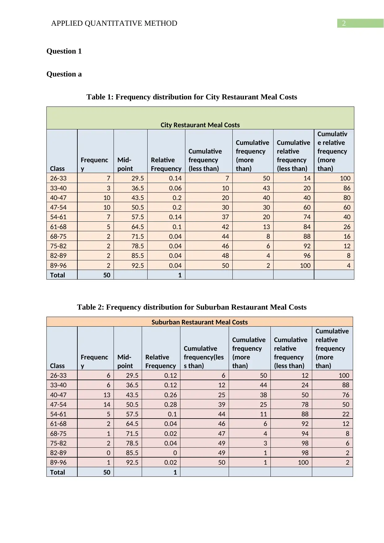
Table 1: Frequency distribution for City Restaurant Meal Costs
City Restaurant Meal Costs
Class
Frequenc
y
Mid-
point
Relative
Frequency
Cumulative
frequency
(less than)
Cumulative
frequency
(more
than)
Cumulative
relative
frequency
(less than)
Cumulativ
e relative
frequency
(more
than)
26-33 7 29.5 0.14 7 50 14 100
33-40 3 36.5 0.06 10 43 20 86
40-47 10 43.5 0.2 20 40 40 80
47-54 10 50.5 0.2 30 30 60 60
54-61 7 57.5 0.14 37 20 74 40
61-68 5 64.5 0.1 42 13 84 26
68-75 2 71.5 0.04 44 8 88 16
75-82 2 78.5 0.04 46 6 92 12
82-89 2 85.5 0.04 48 4 96 8
89-96 2 92.5 0.04 50 2 100 4
Total 50 1
Table 2: Frequency distribution for Suburban Restaurant Meal Costs
Suburban Restaurant Meal Costs
Class
Frequenc
y
Mid-
point
Relative
Frequency
Cumulative
frequency(les
s than)
Cumulative
frequency
(more
than)
Cumulative
relative
frequency
(less than)
Cumulative
relative
frequency
(more
than)
26-33 6 29.5 0.12 6 50 12 100
33-40 6 36.5 0.12 12 44 24 88
40-47 13 43.5 0.26 25 38 50 76
47-54 14 50.5 0.28 39 25 78 50
54-61 5 57.5 0.1 44 11 88 22
61-68 2 64.5 0.04 46 6 92 12
68-75 1 71.5 0.02 47 4 94 8
75-82 2 78.5 0.04 49 3 98 6
82-89 0 85.5 0 49 1 98 2
89-96 1 92.5 0.02 50 1 100 2
Total 50 1
Question 1
Question a
Table 1: Frequency distribution for City Restaurant Meal Costs
City Restaurant Meal Costs
Class
Frequenc
y
Mid-
point
Relative
Frequency
Cumulative
frequency
(less than)
Cumulative
frequency
(more
than)
Cumulative
relative
frequency
(less than)
Cumulativ
e relative
frequency
(more
than)
26-33 7 29.5 0.14 7 50 14 100
33-40 3 36.5 0.06 10 43 20 86
40-47 10 43.5 0.2 20 40 40 80
47-54 10 50.5 0.2 30 30 60 60
54-61 7 57.5 0.14 37 20 74 40
61-68 5 64.5 0.1 42 13 84 26
68-75 2 71.5 0.04 44 8 88 16
75-82 2 78.5 0.04 46 6 92 12
82-89 2 85.5 0.04 48 4 96 8
89-96 2 92.5 0.04 50 2 100 4
Total 50 1
Table 2: Frequency distribution for Suburban Restaurant Meal Costs
Suburban Restaurant Meal Costs
Class
Frequenc
y
Mid-
point
Relative
Frequency
Cumulative
frequency(les
s than)
Cumulative
frequency
(more
than)
Cumulative
relative
frequency
(less than)
Cumulative
relative
frequency
(more
than)
26-33 6 29.5 0.12 6 50 12 100
33-40 6 36.5 0.12 12 44 24 88
40-47 13 43.5 0.26 25 38 50 76
47-54 14 50.5 0.28 39 25 78 50
54-61 5 57.5 0.1 44 11 88 22
61-68 2 64.5 0.04 46 6 92 12
68-75 1 71.5 0.02 47 4 94 8
75-82 2 78.5 0.04 49 3 98 6
82-89 0 85.5 0 49 1 98 2
89-96 1 92.5 0.02 50 1 100 2
Total 50 1
⊘ This is a preview!⊘
Do you want full access?
Subscribe today to unlock all pages.
Trusted by 1+ million students worldwide
3APPLIED QUANTITATIVE METHOD
Question b
26-33 33-40 40-47 47-54 54-61 61-68 68-75 75-82 82-89 89-96
0
2
4
6
8
10
12
Histogram for City Restaurant Meal Costs
Class
Frequency
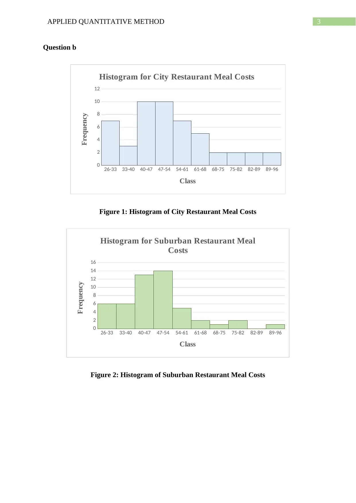
Figure 1: Histogram of City Restaurant Meal Costs
26-33 33-40 40-47 47-54 54-61 61-68 68-75 75-82 82-89 89-96
0
2
4
6
8
10
12
14
16
Histogram for Suburban Restaurant Meal
Costs
Class
Frequency
Figure 2: Histogram of Suburban Restaurant Meal Costs
Question b
26-33 33-40 40-47 47-54 54-61 61-68 68-75 75-82 82-89 89-96
0
2
4
6
8
10
12
Histogram for City Restaurant Meal Costs
Class
Frequency
Figure 1: Histogram of City Restaurant Meal Costs
26-33 33-40 40-47 47-54 54-61 61-68 68-75 75-82 82-89 89-96
0
2
4
6
8
10
12
14
16
Histogram for Suburban Restaurant Meal
Costs
Class
Frequency
Figure 2: Histogram of Suburban Restaurant Meal Costs
Paraphrase This Document
Need a fresh take? Get an instant paraphrase of this document with our AI Paraphraser
4APPLIED QUANTITATIVE METHOD
Question c
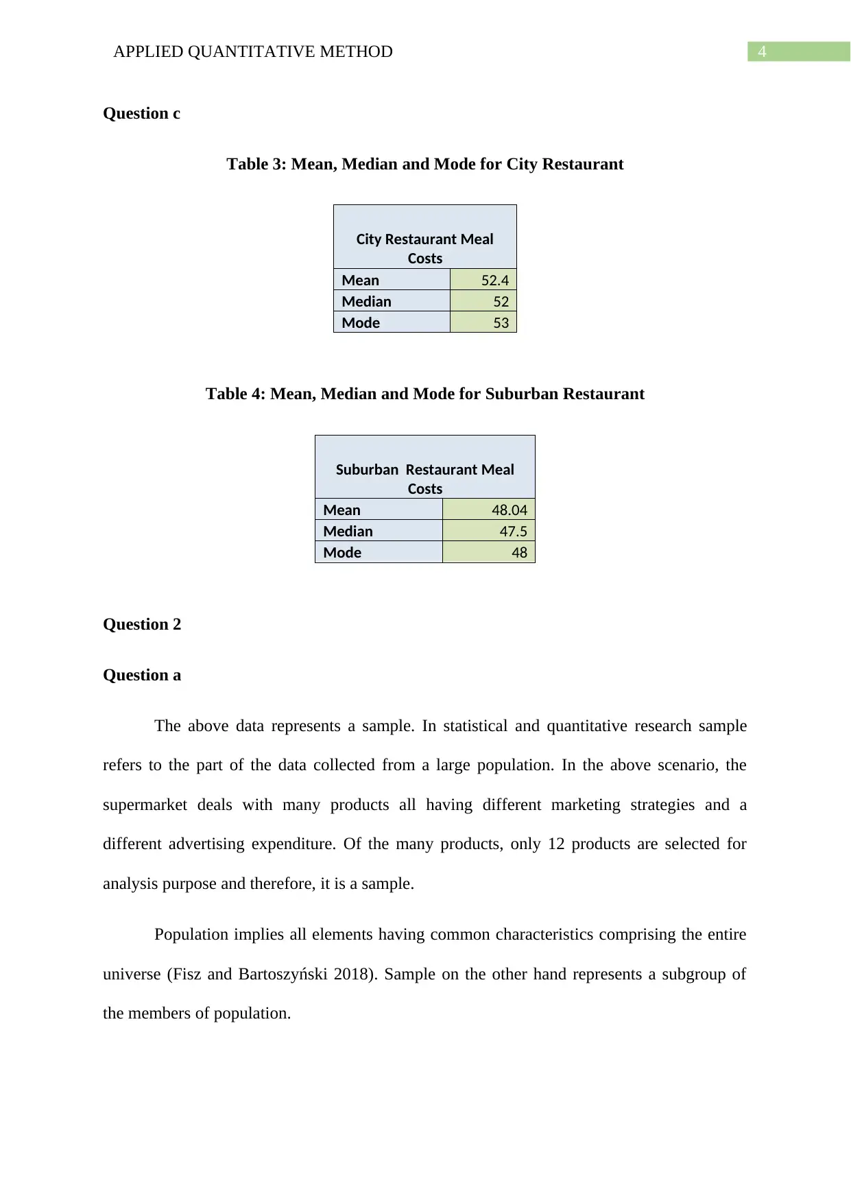
Table 3: Mean, Median and Mode for City Restaurant
City Restaurant Meal
Costs
Mean 52.4
Median 52
Mode 53
Table 4: Mean, Median and Mode for Suburban Restaurant
Suburban Restaurant Meal
Costs
Mean 48.04
Median 47.5
Mode 48
Question 2
Question a
The above data represents a sample. In statistical and quantitative research sample
refers to the part of the data collected from a large population. In the above scenario, the
supermarket deals with many products all having different marketing strategies and a
different advertising expenditure. Of the many products, only 12 products are selected for
analysis purpose and therefore, it is a sample.
Population implies all elements having common characteristics comprising the entire
universe (Fisz and Bartoszyński 2018). Sample on the other hand represents a subgroup of
the members of population.
Question c
Table 3: Mean, Median and Mode for City Restaurant
City Restaurant Meal
Costs
Mean 52.4
Median 52
Mode 53
Table 4: Mean, Median and Mode for Suburban Restaurant
Suburban Restaurant Meal
Costs
Mean 48.04
Median 47.5
Mode 48
Question 2
Question a
The above data represents a sample. In statistical and quantitative research sample
refers to the part of the data collected from a large population. In the above scenario, the
supermarket deals with many products all having different marketing strategies and a
different advertising expenditure. Of the many products, only 12 products are selected for
analysis purpose and therefore, it is a sample.
Population implies all elements having common characteristics comprising the entire
universe (Fisz and Bartoszyński 2018). Sample on the other hand represents a subgroup of
the members of population.
5APPLIED QUANTITATIVE METHOD
Question b
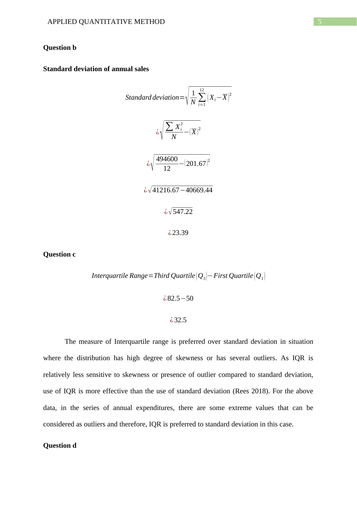
Standard deviation of annual sales
Standard deviation= √ 1
N ∑
i=1
12
( Xi −X ) 2
¿ √ ∑ Xi
2
N − ( X ) 2
¿ √ 494600
12 − ( 201.67 ) 2
¿ √41216.67−40669.44
¿ √ 547.22
¿ 23.39
Question c
Interquartile Range=Third Quartile ( Q3 ) −First Quartile ( Q1 )
¿ 82.5−50
¿ 32.5
The measure of Interquartile range is preferred over standard deviation in situation
where the distribution has high degree of skewness or has several outliers. As IQR is
relatively less sensitive to skewness or presence of outlier compared to standard deviation,
use of IQR is more effective than the use of standard deviation (Rees 2018). For the above
data, in the series of annual expenditures, there are some extreme values that can be
considered as outliers and therefore, IQR is preferred to standard deviation in this case.
Question d
Question b
Standard deviation of annual sales
Standard deviation= √ 1
N ∑
i=1
12
( Xi −X ) 2
¿ √ ∑ Xi
2
N − ( X ) 2
¿ √ 494600
12 − ( 201.67 ) 2
¿ √41216.67−40669.44
¿ √ 547.22
¿ 23.39
Question c
Interquartile Range=Third Quartile ( Q3 ) −First Quartile ( Q1 )
¿ 82.5−50
¿ 32.5
The measure of Interquartile range is preferred over standard deviation in situation
where the distribution has high degree of skewness or has several outliers. As IQR is
relatively less sensitive to skewness or presence of outlier compared to standard deviation,
use of IQR is more effective than the use of standard deviation (Rees 2018). For the above
data, in the series of annual expenditures, there are some extreme values that can be
considered as outliers and therefore, IQR is preferred to standard deviation in this case.
Question d
⊘ This is a preview!⊘
Do you want full access?
Subscribe today to unlock all pages.
Trusted by 1+ million students worldwide
6APPLIED QUANTITATIVE METHOD
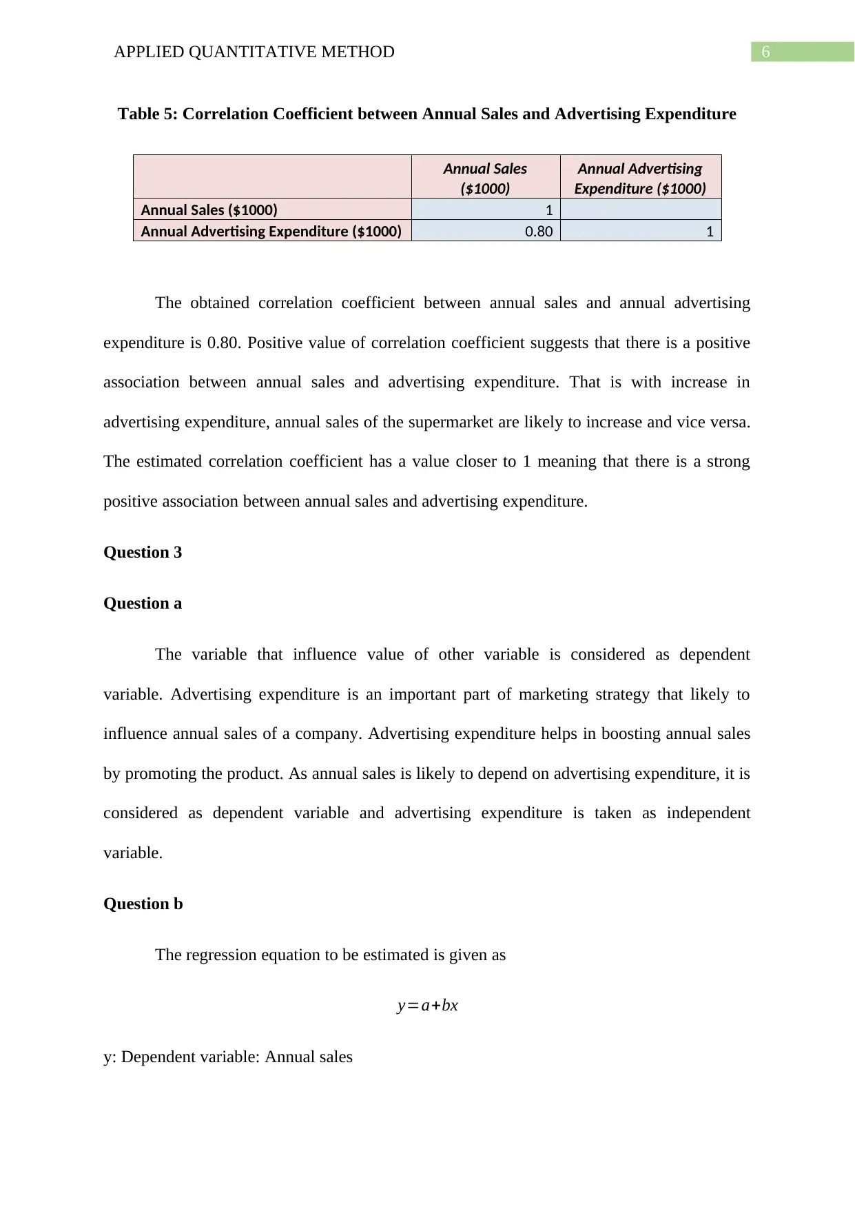
Table 5: Correlation Coefficient between Annual Sales and Advertising Expenditure
Annual Sales
($1000)
Annual Advertising
Expenditure ($1000)
Annual Sales ($1000) 1
Annual Advertising Expenditure ($1000) 0.80 1
The obtained correlation coefficient between annual sales and annual advertising
expenditure is 0.80. Positive value of correlation coefficient suggests that there is a positive
association between annual sales and advertising expenditure. That is with increase in
advertising expenditure, annual sales of the supermarket are likely to increase and vice versa.
The estimated correlation coefficient has a value closer to 1 meaning that there is a strong
positive association between annual sales and advertising expenditure.
Question 3
Question a
The variable that influence value of other variable is considered as dependent
variable. Advertising expenditure is an important part of marketing strategy that likely to
influence annual sales of a company. Advertising expenditure helps in boosting annual sales
by promoting the product. As annual sales is likely to depend on advertising expenditure, it is
considered as dependent variable and advertising expenditure is taken as independent
variable.
Question b
The regression equation to be estimated is given as
y=a+bx
y: Dependent variable: Annual sales
Paraphrase This Document
Need a fresh take? Get an instant paraphrase of this document with our AI Paraphraser
7APPLIED QUANTITATIVE METHOD
x: Independent variable: Advertising expenditure
a: Intercept
b: Slope coefficient
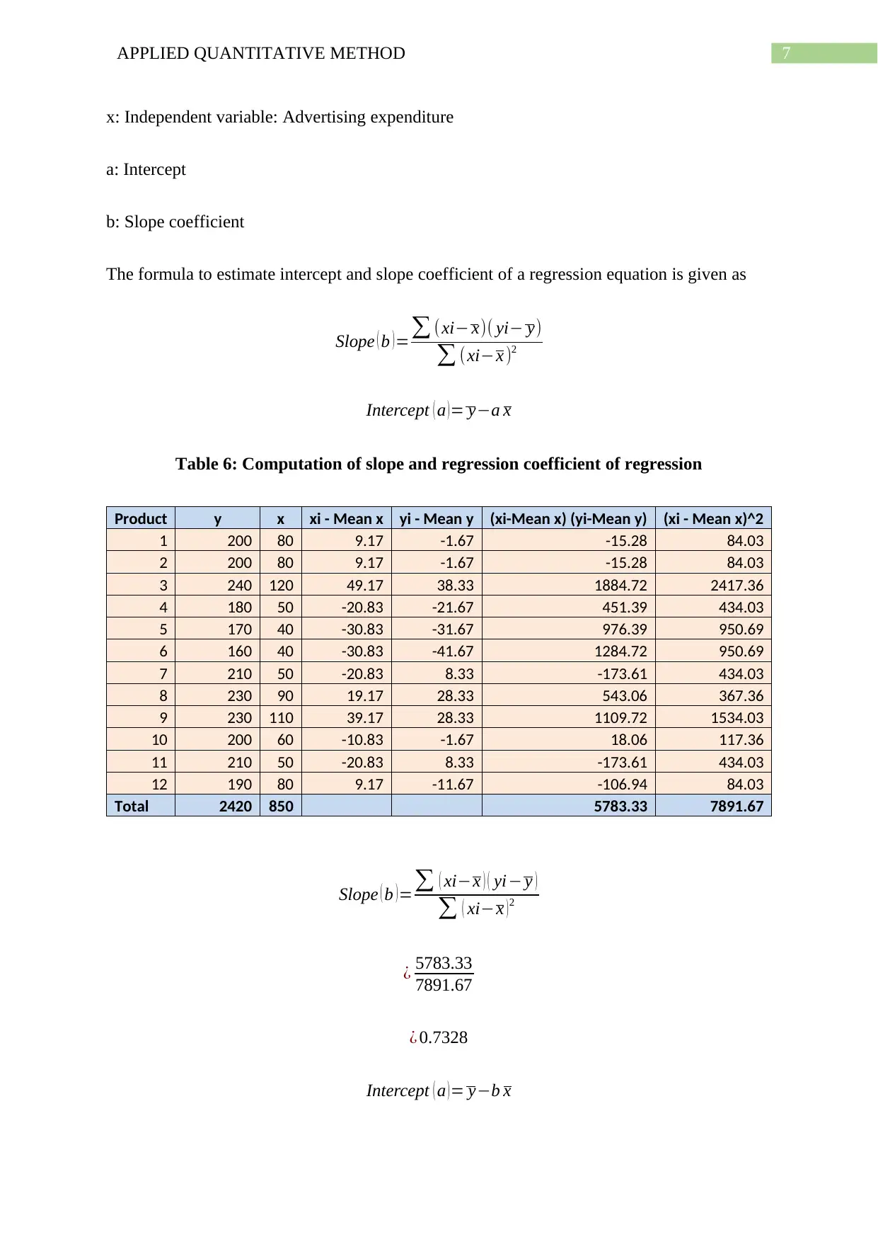
The formula to estimate intercept and slope coefficient of a regression equation is given as
Slope ( b )=∑ (xi− x)( yi− y)
∑ (xi−x )2
Intercept ( a )= y−a x
Table 6: Computation of slope and regression coefficient of regression
Product y x xi - Mean x yi - Mean y (xi-Mean x) (yi-Mean y) (xi - Mean x)^2
1 200 80 9.17 -1.67 -15.28 84.03
2 200 80 9.17 -1.67 -15.28 84.03
3 240 120 49.17 38.33 1884.72 2417.36
4 180 50 -20.83 -21.67 451.39 434.03
5 170 40 -30.83 -31.67 976.39 950.69
6 160 40 -30.83 -41.67 1284.72 950.69
7 210 50 -20.83 8.33 -173.61 434.03
8 230 90 19.17 28.33 543.06 367.36
9 230 110 39.17 28.33 1109.72 1534.03
10 200 60 -10.83 -1.67 18.06 117.36
11 210 50 -20.83 8.33 -173.61 434.03
12 190 80 9.17 -11.67 -106.94 84.03
Total 2420 850 5783.33 7891.67
Slope ( b )=∑ ( xi−x ) ( yi− y )
∑ ( xi−x )2
¿ 5783.33
7891.67
¿ 0.7328
Intercept ( a ) = y−b x
x: Independent variable: Advertising expenditure
a: Intercept
b: Slope coefficient
The formula to estimate intercept and slope coefficient of a regression equation is given as
Slope ( b )=∑ (xi− x)( yi− y)
∑ (xi−x )2
Intercept ( a )= y−a x
Table 6: Computation of slope and regression coefficient of regression
Product y x xi - Mean x yi - Mean y (xi-Mean x) (yi-Mean y) (xi - Mean x)^2
1 200 80 9.17 -1.67 -15.28 84.03
2 200 80 9.17 -1.67 -15.28 84.03
3 240 120 49.17 38.33 1884.72 2417.36
4 180 50 -20.83 -21.67 451.39 434.03
5 170 40 -30.83 -31.67 976.39 950.69
6 160 40 -30.83 -41.67 1284.72 950.69
7 210 50 -20.83 8.33 -173.61 434.03
8 230 90 19.17 28.33 543.06 367.36
9 230 110 39.17 28.33 1109.72 1534.03
10 200 60 -10.83 -1.67 18.06 117.36
11 210 50 -20.83 8.33 -173.61 434.03
12 190 80 9.17 -11.67 -106.94 84.03
Total 2420 850 5783.33 7891.67
Slope ( b )=∑ ( xi−x ) ( yi− y )
∑ ( xi−x )2
¿ 5783.33
7891.67
¿ 0.7328
Intercept ( a ) = y−b x
8APPLIED QUANTITATIVE METHOD
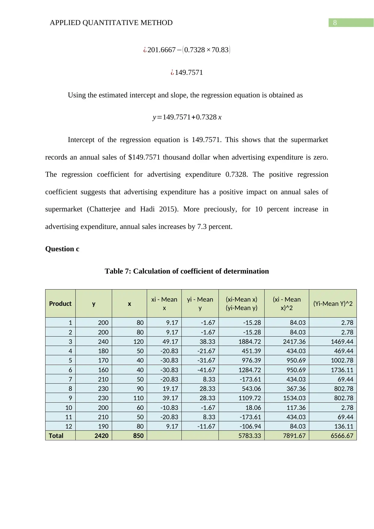
¿ 201.6667− ( 0.7328 ×70.83 )
¿ 149.7571
Using the estimated intercept and slope, the regression equation is obtained as
y=149.7571+0.7328 x
Intercept of the regression equation is 149.7571. This shows that the supermarket
records an annual sales of $149.7571 thousand dollar when advertising expenditure is zero.
The regression coefficient for advertising expenditure 0.7328. The positive regression
coefficient suggests that advertising expenditure has a positive impact on annual sales of
supermarket (Chatterjee and Hadi 2015). More preciously, for 10 percent increase in
advertising expenditure, annual sales increases by 7.3 percent.
Question c
Table 7: Calculation of coefficient of determination
Product y x xi - Mean
x
yi - Mean
y
(xi-Mean x)
(yi-Mean y)
(xi - Mean
x)^2 (Yi-Mean Y)^2
1 200 80 9.17 -1.67 -15.28 84.03 2.78
2 200 80 9.17 -1.67 -15.28 84.03 2.78
3 240 120 49.17 38.33 1884.72 2417.36 1469.44
4 180 50 -20.83 -21.67 451.39 434.03 469.44
5 170 40 -30.83 -31.67 976.39 950.69 1002.78
6 160 40 -30.83 -41.67 1284.72 950.69 1736.11
7 210 50 -20.83 8.33 -173.61 434.03 69.44
8 230 90 19.17 28.33 543.06 367.36 802.78
9 230 110 39.17 28.33 1109.72 1534.03 802.78
10 200 60 -10.83 -1.67 18.06 117.36 2.78
11 210 50 -20.83 8.33 -173.61 434.03 69.44
12 190 80 9.17 -11.67 -106.94 84.03 136.11
Total 2420 850 5783.33 7891.67 6566.67
⊘ This is a preview!⊘
Do you want full access?
Subscribe today to unlock all pages.
Trusted by 1+ million students worldwide
9APPLIED QUANTITATIVE METHOD
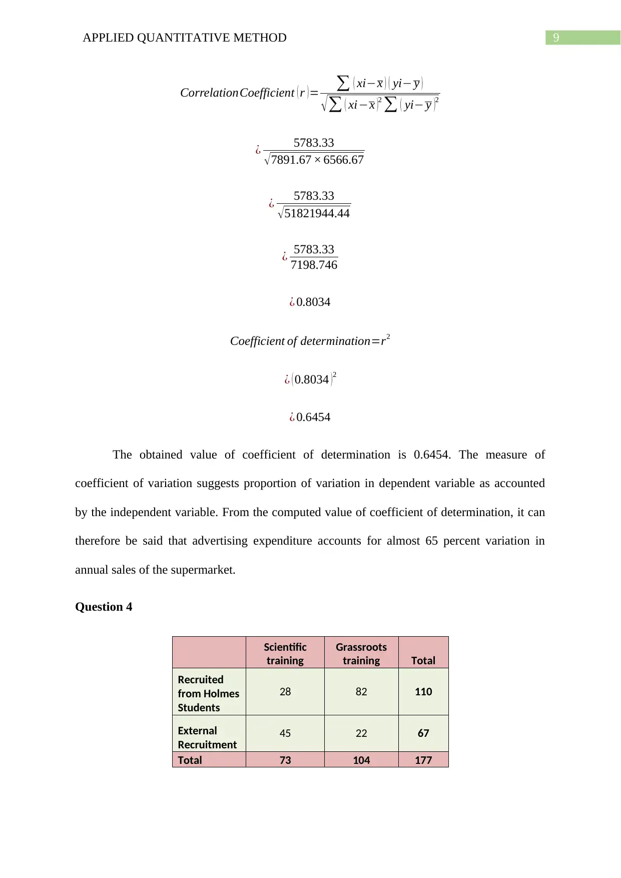
CorrelationCoefficient ( r ) = ∑ ( xi−x ) ( yi− y )
√ ∑ ( xi−x )2
∑ ( yi− y )2
¿ 5783.33
√7891.67 × 6566.67
¿ 5783.33
√51821944.44
¿ 5783.33
7198.746
¿ 0.8034
Coefficient of determination=r2
¿ ( 0.8034 ) 2
¿ 0.6454
The obtained value of coefficient of determination is 0.6454. The measure of
coefficient of variation suggests proportion of variation in dependent variable as accounted
by the independent variable. From the computed value of coefficient of determination, it can
therefore be said that advertising expenditure accounts for almost 65 percent variation in
annual sales of the supermarket.
Question 4
Scientific
training
Grassroots
training Total
Recruited
from Holmes
Students
28 82 110
External
Recruitment 45 22 67
Total 73 104 177
Paraphrase This Document
Need a fresh take? Get an instant paraphrase of this document with our AI Paraphraser
10APPLIED QUANTITATIVE METHOD
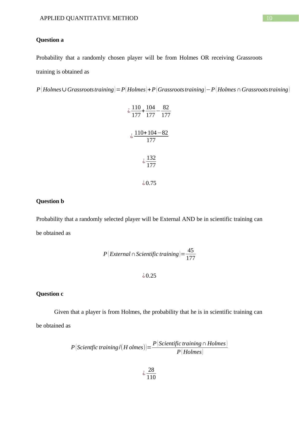
Question a
Probability that a randomly chosen player will be from Holmes OR receiving Grassroots
training is obtained as
P ( Holmes∪Grassroots training ) =P ( Holmes ) + P ( Grassroots training )−P ( Holmes ∩Grassroots training )
¿ 110
177 + 104
177 − 82
177
¿ 110+ 104−82
177
¿ 132
177
¿ 0.75
Question b
Probability that a randomly selected player will be External AND be in scientific training can
be obtained as
P ( External ∩Scientific training )= 45
177
¿ 0.25
Question c
Given that a player is from Holmes, the probability that he is in scientific training can
be obtained as
P ( Scientfic training /(H olmes) )= P ( Scientific training ∩ Holmes )
P ( Holmes )
¿ 28
110
11APPLIED QUANTITATIVE METHOD
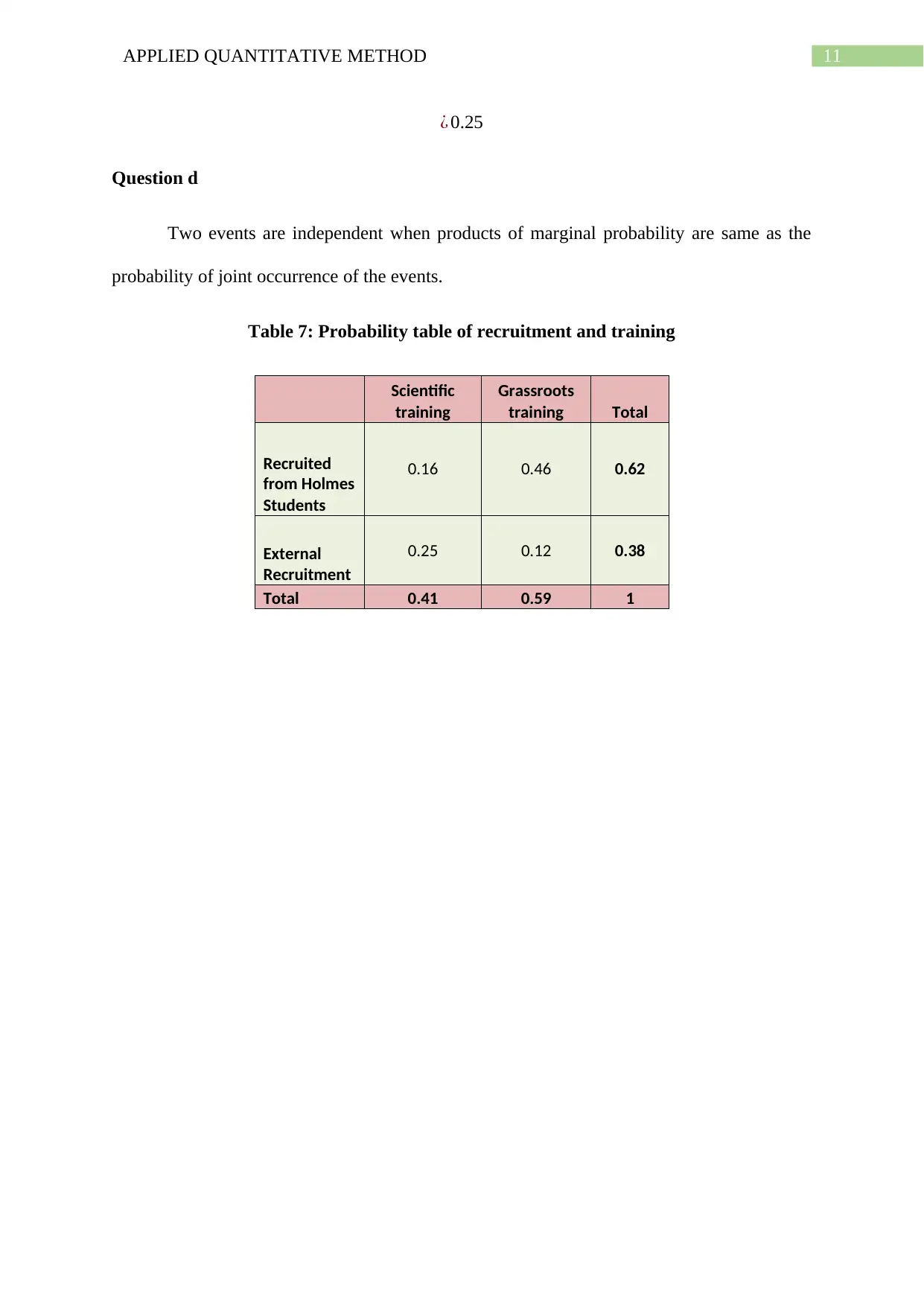
¿ 0.25
Question d
Two events are independent when products of marginal probability are same as the
probability of joint occurrence of the events.
Table 7: Probability table of recruitment and training
Scientific
training
Grassroots
training Total
Recruited
from Holmes
Students
0.16 0.46 0.62
External
Recruitment
0.25 0.12 0.38
Total 0.41 0.59 1
⊘ This is a preview!⊘
Do you want full access?
Subscribe today to unlock all pages.
Trusted by 1+ million students worldwide
1 out of 16


Your All-in-One AI-Powered Toolkit for Academic Success.
+13062052269
info@desklib.com
Available 24*7 on WhatsApp / Email
![[object Object]](/_next/static/media/star-bottom.7253800d.svg)
Unlock your academic potential
Copyright © 2020–2026 A2Z Services. All Rights Reserved. Developed and managed by ZUCOL.