Group Assignment: Applied Quantitative Methods for HA1011, T2 2018

This assignment solution addresses a range of applied quantitative methods, starting with frequency distribution, histograms, and calculations of mean, median, and mode. It then delves into descriptive statistics, including standard deviation and interquartile range calculations for sample data. Th...Read More

Applied quantitative methods
Applied quantitative methods
Student name:
Student number:
Tutor name:

Applied quantitative methods
QUESTION 1
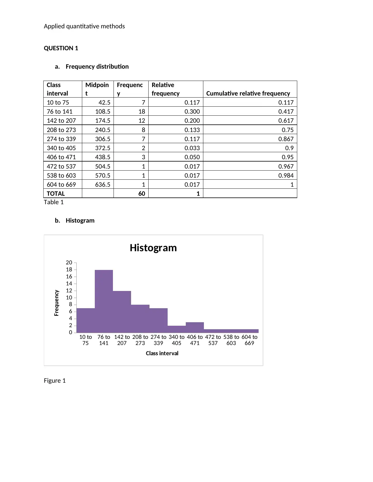
a. Frequency distribution
Class
interval
Midpoin
t
Frequenc
y
Relative
frequency Cumulative relative frequency
10 to 75 42.5 7 0.117 0.117
76 to 141 108.5 18 0.300 0.417
142 to 207 174.5 12 0.200 0.617
208 to 273 240.5 8 0.133 0.75
274 to 339 306.5 7 0.117 0.867
340 to 405 372.5 2 0.033 0.9
406 to 471 438.5 3 0.050 0.95
472 to 537 504.5 1 0.017 0.967
538 to 603 570.5 1 0.017 0.984
604 to 669 636.5 1 0.017 1
TOTAL 60 1
Table 1
b. Histogram
10 to
75 76 to
141 142 to
207 208 to
273 274 to
339 340 to
405 406 to
471 472 to
537 538 to
603 604 to
669
0
2
4
6
8
10
12
14
16
18
20
Histogram
Class interval
Frequency
Figure 1

Applied quantitative methods
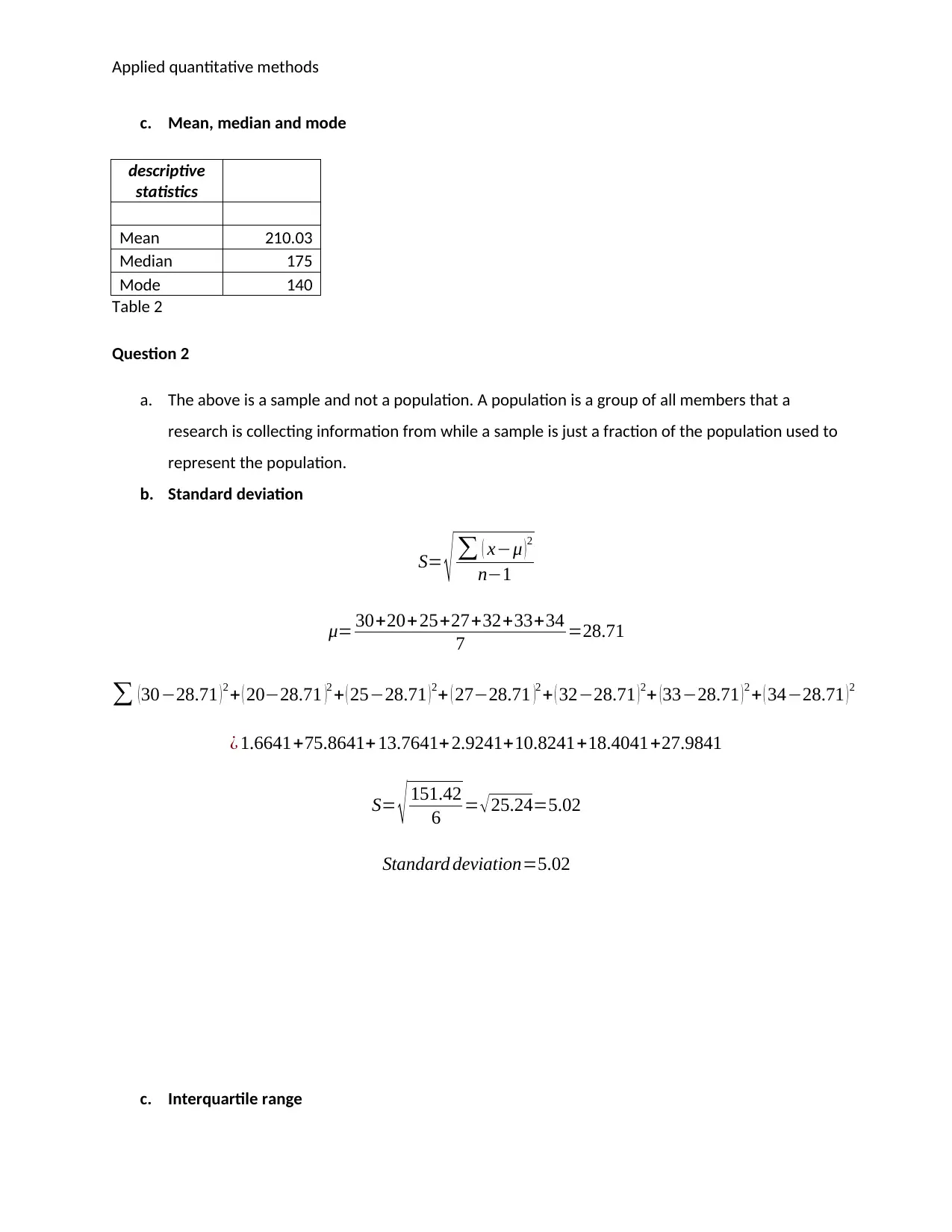
c. Mean, median and mode
descriptive
statistics
Mean 210.03
Median 175
Mode 140
Table 2
Question 2
a. The above is a sample and not a population. A population is a group of all members that a
research is collecting information from while a sample is just a fraction of the population used to
represent the population.
b. Standard deviation
S= √ ∑ ( x−μ )2
n−1
μ= 30+20+25+27+32+33+34
7 =28.71
∑ (30−28.71 )2 + ( 20−28.71 )2 + ( 25−28.71 )2+ ( 27−28.71 )2 + ( 32−28.71 )2+ (33−28.71 )2 + ( 34−28.71 )2
¿ 1.6641+75.8641+ 13.7641+2.9241+10.8241+18.4041+27.9841
S= √ 151.42
6 = √ 25.24=5.02
Standard deviation=5.02
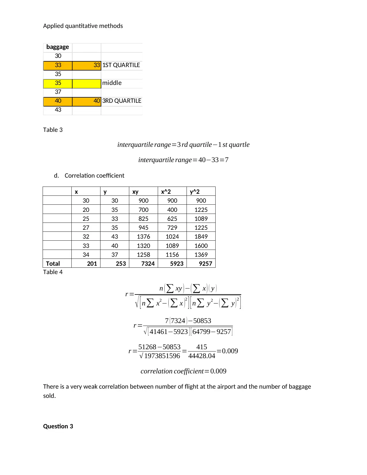
c. Interquartile range

Applied quantitative methods
baggage
30
33 33 1ST QUARTILE
35
35 middle
37
40 40 3RD QUARTILE
43
Table 3
interquartile range=3 rd quartile−1 st quartle
interquartile range=40−33=7
d. Correlation coefficient
x y xy x^2 y^2
30 30 900 900 900
20 35 700 400 1225
25 33 825 625 1089
27 35 945 729 1225
32 43 1376 1024 1849
33 40 1320 1089 1600
34 37 1258 1156 1369
Total 201 253 7324 5923 9257
Table 4
r = n ( ∑ xy ) − ( ∑ x ) ( y )
√ [ n∑ x2− ( ∑ x )
2
] [ n∑ y2− ( ∑ y ) 2
]
r = 7 (7324 )−50853
√ [ 41461−5923 ] [ 64799−9257 ]
r =51268−50853
√ 1973851596 = 415
44428.04 =0.009
correlation coefficient=0.009
There is a very weak correlation between number of flight at the airport and the number of baggage
sold.
Question 3

Applied quantitative methods
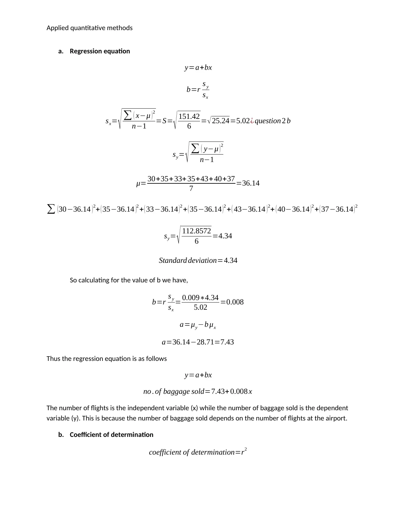
a. Regression equation
y=a+bx
b=r s y
sx
sx= √ ∑ ( x−μ ) 2
n−1 =S= √ 151.42
6 = √ 25.24=5.02¿ question 2 b
sy= √ ∑ ( y−μ ) 2
n−1
μ= 30+35+33+35+43+ 40+37
7 =36.14
∑ (30−36.14 )2+ ( 35−36.14 )2 + ( 33−36.14 )2 + ( 35−36.14 )2 + ( 43−36.14 )2+ ( 40−36.14 )2 + ( 37−36.14 )2
sy= √ 112.8572
6 =4.34
Standard deviation=4.34
So calculating for the value of b we have,
b=r s y
sx
= 0.009∗4.34
5.02 =0.008
a=μy−b μx
a=36.14−28.71=7.43
Thus the regression equation is as follows
y=a+bx
no . of baggage sold=7.43+ 0.008 x
The number of flights is the independent variable (x) while the number of baggage sold is the dependent
variable (y). This is because the number of baggage sold depends on the number of flights at the airport.
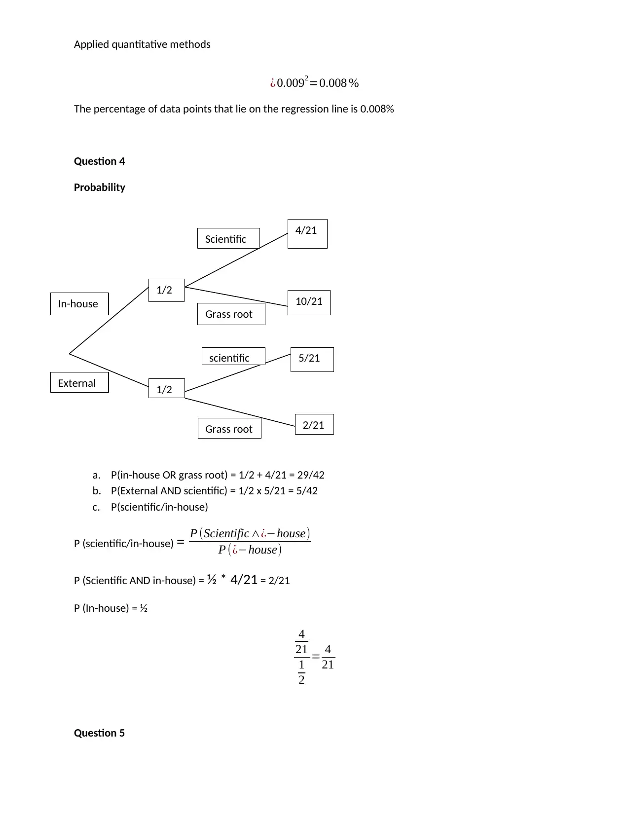
b. Coefficient of determination
coefficient of determination=r2

Applied quantitative methods
¿ 0.0092=0.008 %
The percentage of data points that lie on the regression line is 0.008%
Question 4
Probability
a. P(in-house OR grass root) = 1/2 + 4/21 = 29/42
b. P(External AND scientific) = 1/2 x 5/21 = 5/42
c. P(scientific/in-house)
P (scientific/in-house) = P (Scientific∧¿−house)
P (¿−house)
P (Scientific AND in-house) = ½ * 4/21 = 2/21
P (In-house) = ½
4
21
1
2
= 4
21
Question 5
1/2
1/2
4/21
10/21
5/21
2/21
In-house
External
Scientific
Grass root
Grass root
scientific

Applied quantitative methods
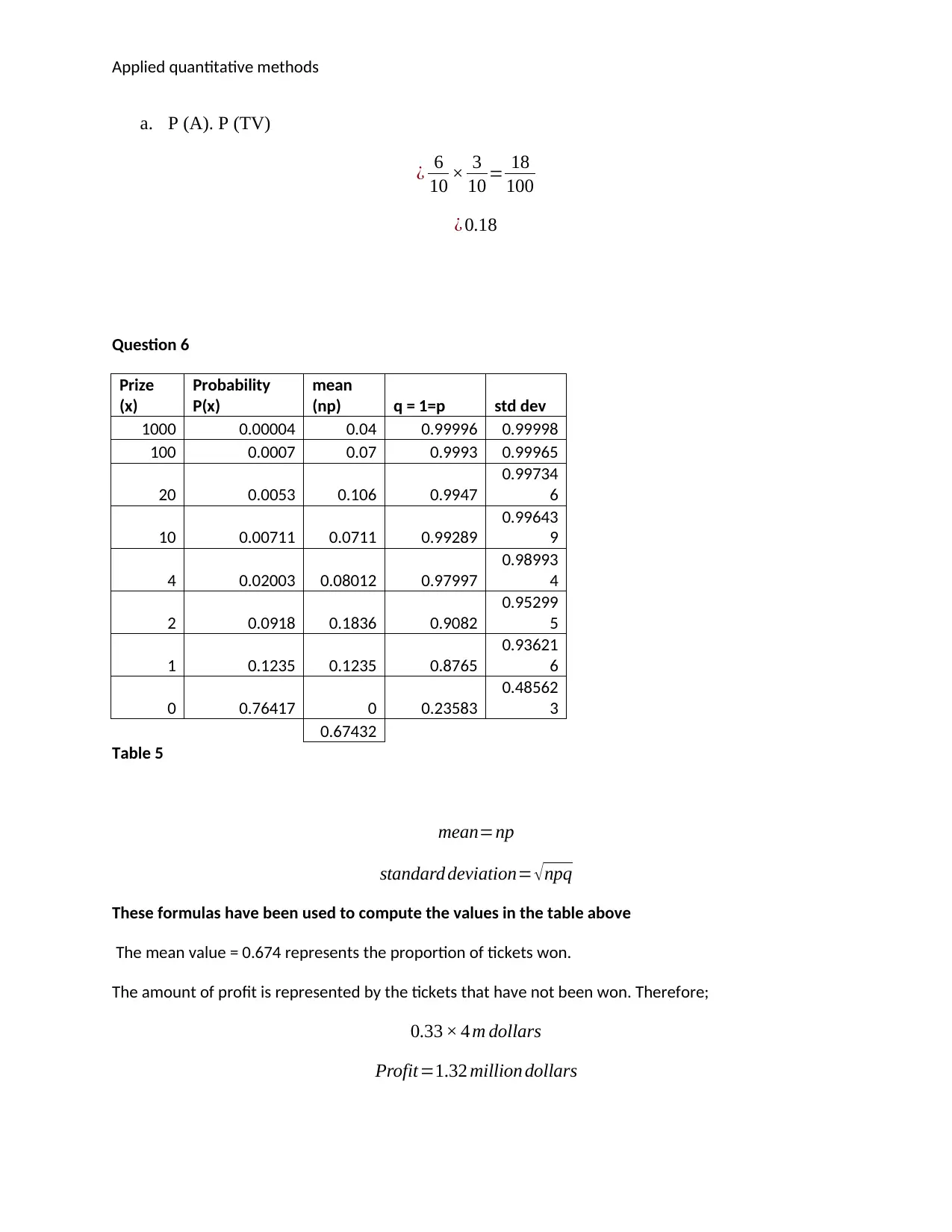
a. P (A). P (TV)
¿ 6
10 × 3
10 = 18
100
¿ 0.18
Question 6
Prize
(x)
Probability
P(x)
mean
(np) q = 1=p std dev
1000 0.00004 0.04 0.99996 0.99998
100 0.0007 0.07 0.9993 0.99965
20 0.0053 0.106 0.9947
0.99734
6
10 0.00711 0.0711 0.99289
0.99643
9
4 0.02003 0.08012 0.97997
0.98993
4
2 0.0918 0.1836 0.9082
0.95299
5
1 0.1235 0.1235 0.8765
0.93621
6
0 0.76417 0 0.23583
0.48562
3
0.67432
Table 5
mean=np
standard deviation= √npq
These formulas have been used to compute the values in the table above
The mean value = 0.674 represents the proportion of tickets won.
The amount of profit is represented by the tickets that have not been won. Therefore;
0.33 × 4 m dollars
Profit=1.32 million dollars

Applied quantitative methods
Question 7
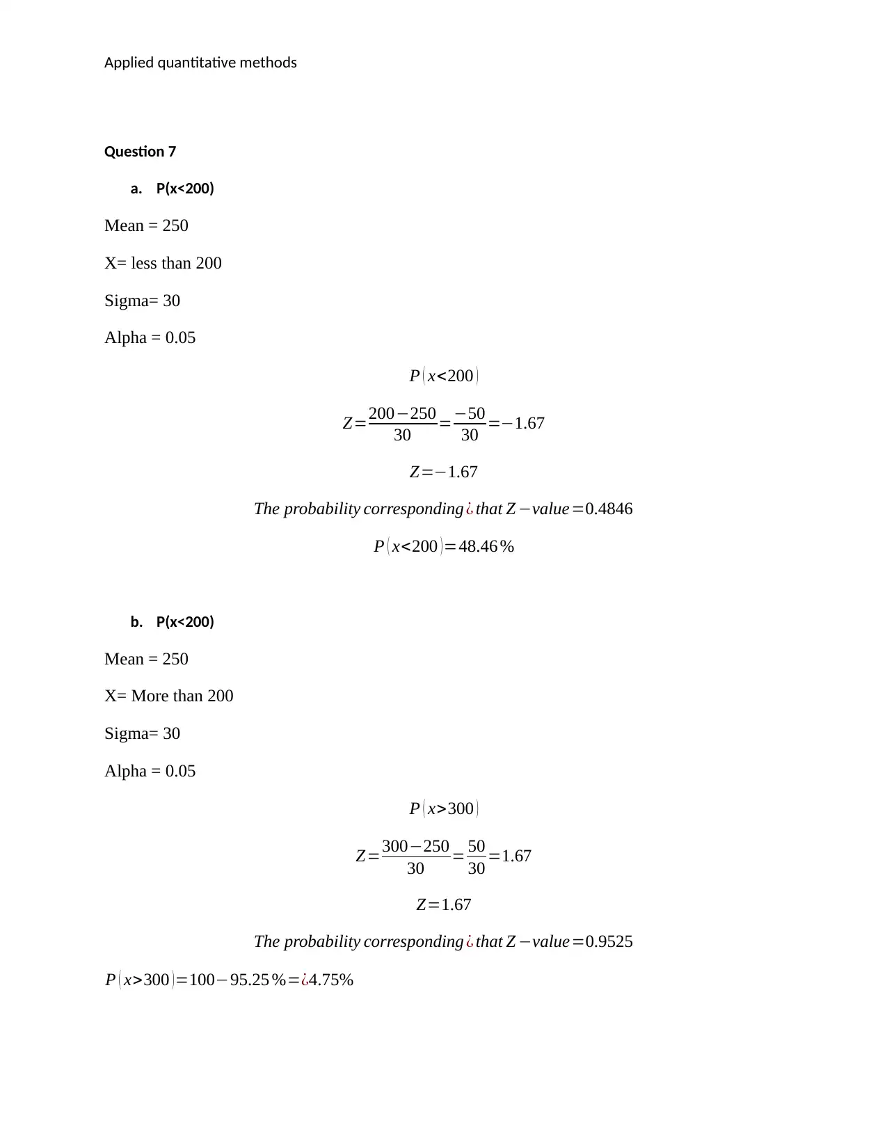
a. P(x<200)
Mean = 250
X= less than 200
Sigma= 30
Alpha = 0.05
P ( x<200 )
Z=200−250
30 =−50
30 =−1.67
Z=−1.67
The probability corresponding ¿ that Z −value=0.4846
P ( x<200 ) =48.46 %
b. P(x<200)
Mean = 250
X= More than 200
Sigma= 30
Alpha = 0.05
P ( x>300 )
Z=300−250
30 = 50
30 =1.67
Z=1.67
The probability corresponding ¿ that Z −value=0.9525
P ( x>300 )=100−95.25 %=¿4.75%

Applied quantitative methods
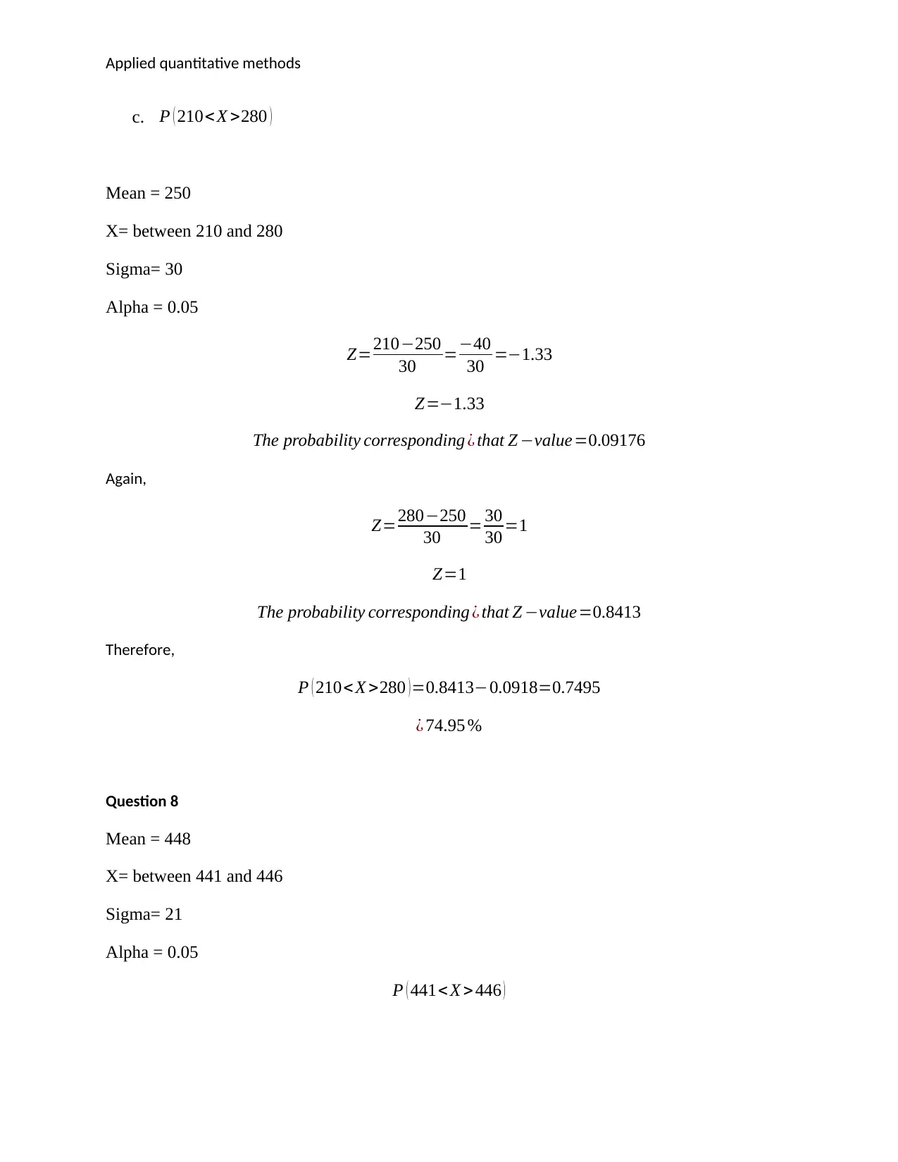
c. P ( 210< X >280 )
Mean = 250
X= between 210 and 280
Sigma= 30
Alpha = 0.05
Z=210−250
30 =−40
30 =−1.33
Z=−1.33
The probability corresponding ¿ that Z −value=0.09176
Again,
Z=280−250
30 = 30
30 =1
Z=1
The probability corresponding ¿ that Z −value=0.8413
Therefore,
P ( 210< X >280 )=0.8413−0.0918=0.7495
¿ 74.95 %
Question 8
Mean = 448
X= between 441 and 446
Sigma= 21
Alpha = 0.05
P ( 441< X >446 )

Applied quantitative methods
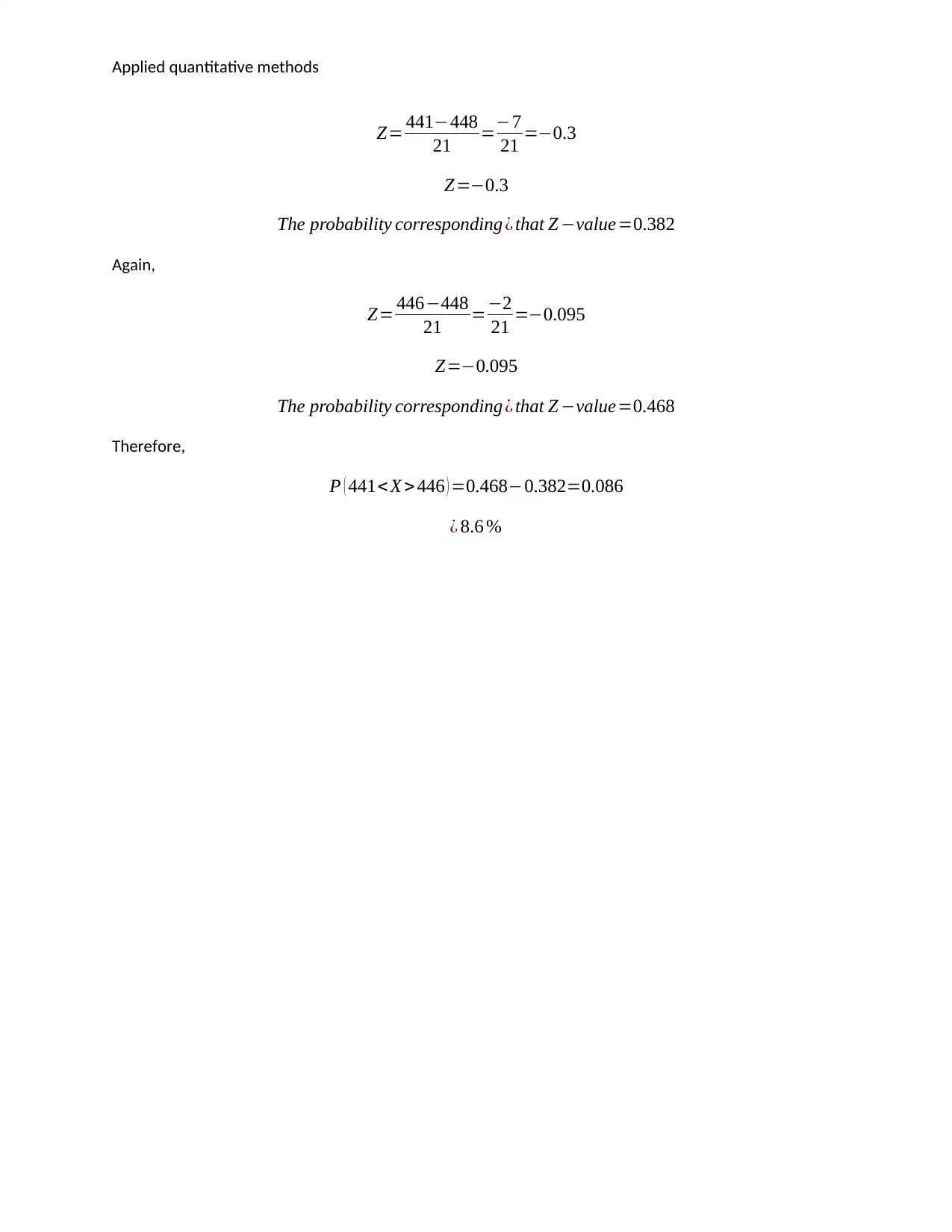
Z= 441−448
21 =−7
21 =−0.3
Z=−0.3
The probability corresponding ¿ that Z −value=0.382
Again,
Z= 446−448
21 =−2
21 =−0.095
Z=−0.095
The probability corresponding ¿ that Z −value=0.468
Therefore,
P ( 441< X >446 ) =0.468−0.382=0.086
¿ 8.6 %