Applied Quantitative Methods HA1011 Assignment Solution T1 2019

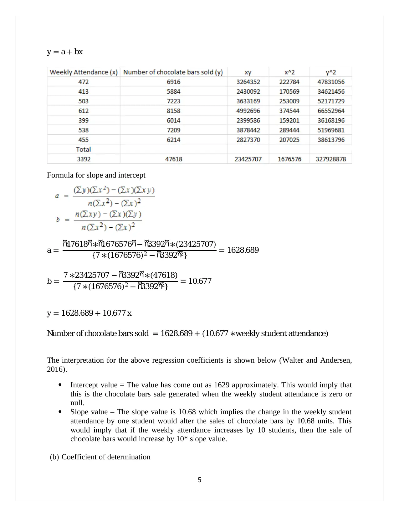
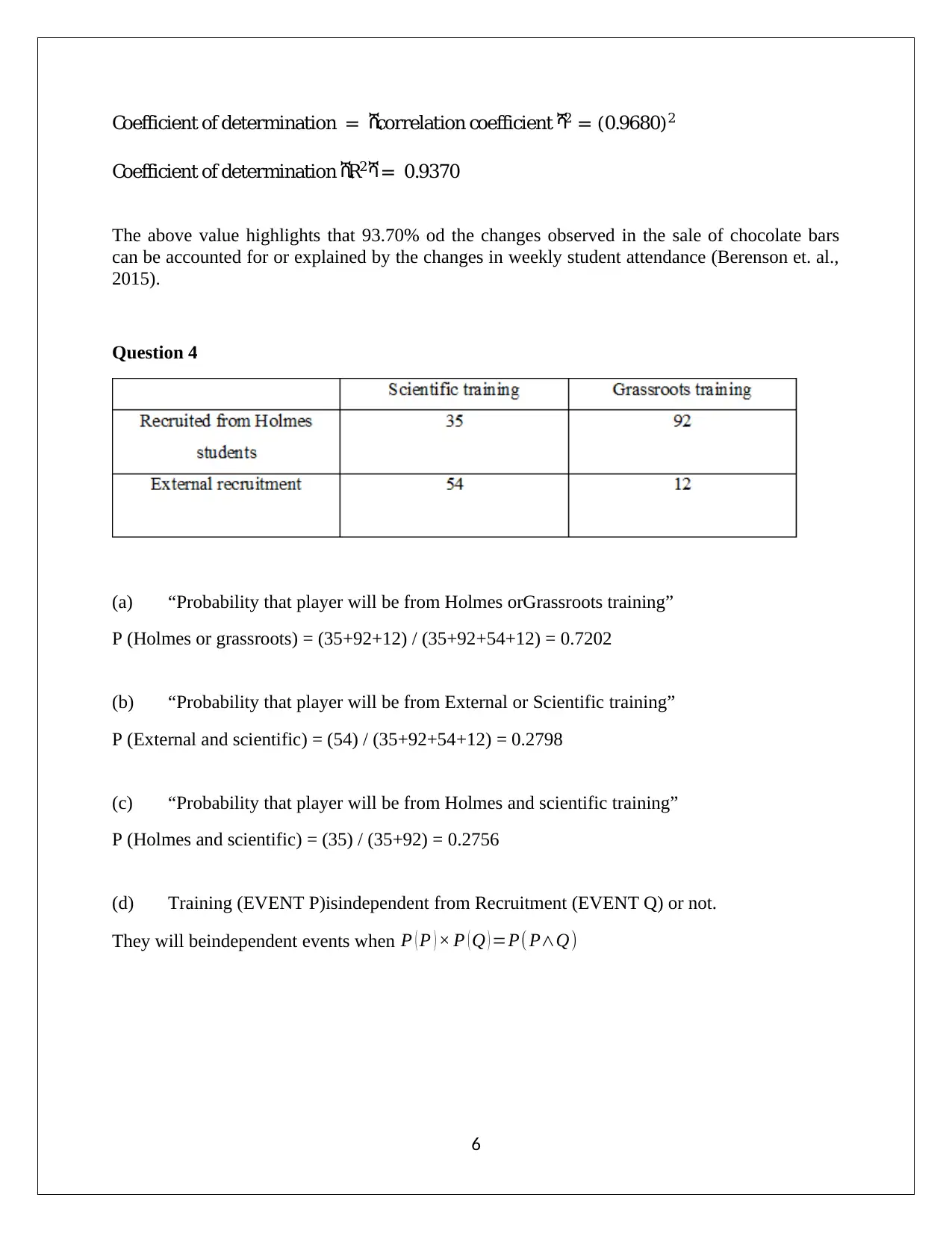
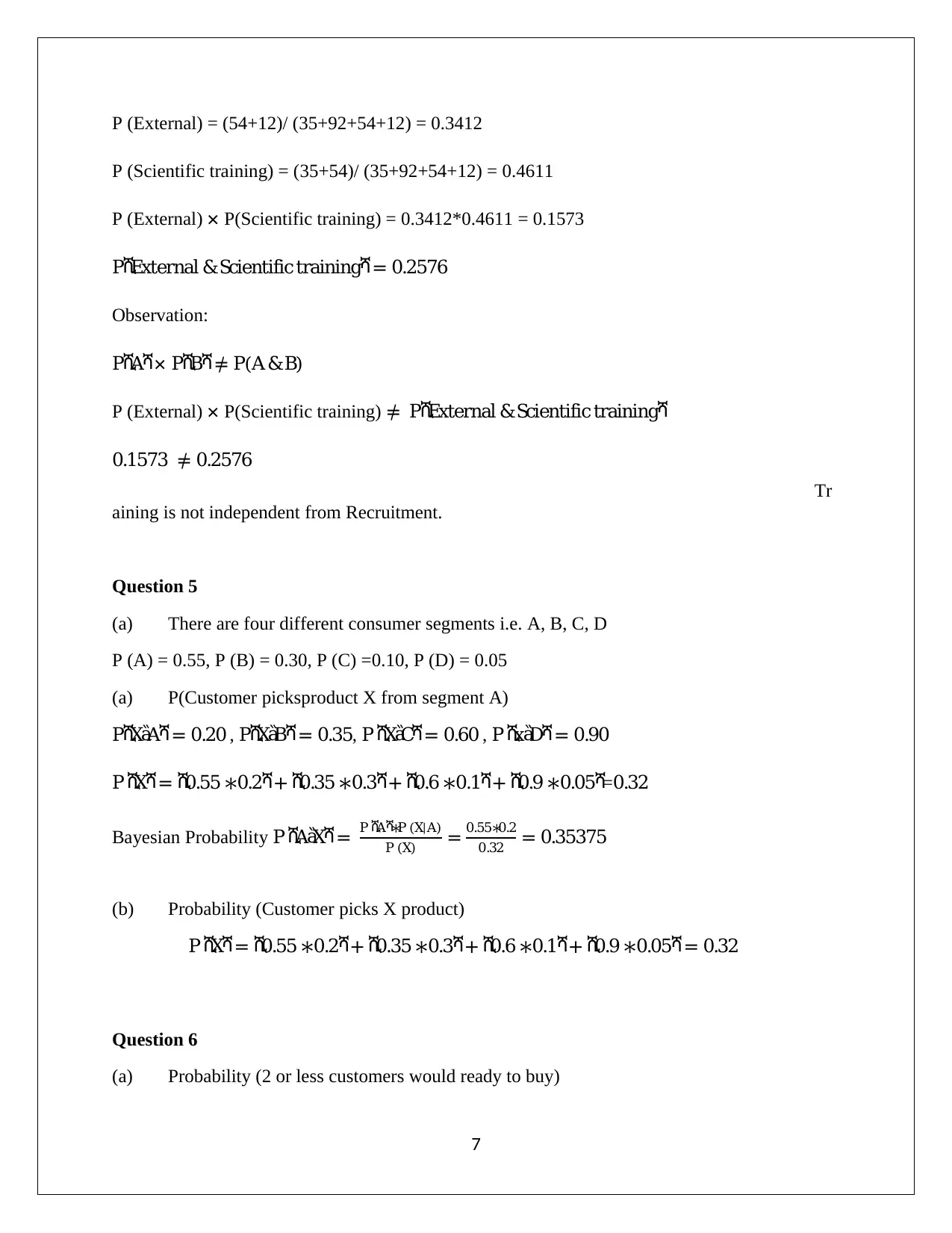
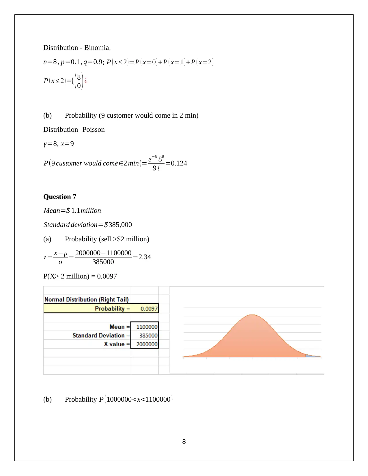
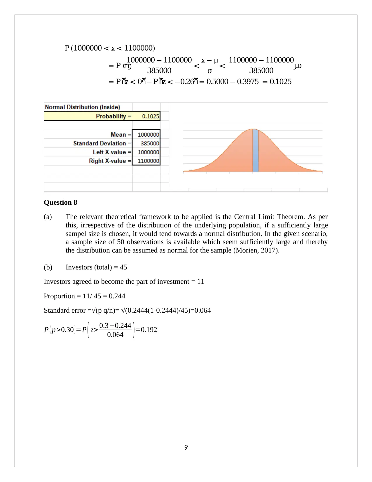
This document presents a comprehensive solution to the HA1011 Applied Quantitative Methods assignment, covering key statistical concepts and techniques. The solution includes calculations and interpretations for frequency distributions, measures of central tendency (mean, median, mo...Read More

APPLIED QUANTITATIVE METHODS
HA1011
Student Name
[Pick the date]

Question 1
(a) Frequency distribution
(b) Frequency histogram
(c) Mean, median and mode of number of passengers computation has been carried out below.
1

2

Mean = 58594/60 = 976.57
M edian= {(60/2) + (60/2+1)}/2 = (30th term +31th term)/2 = (733+862)/2 = 797.5
Maximum repetitionfor a given data value from the given data is for 401
Mode = 401
Question 2
(a) The data that has been provided with regards to weekly attendance and sale of chocolate
pertains only for a handful of weeks and does not pertain to each week in the year. As a
result, the data provided is a sample and not a population.
(b) Standard deviation
Mean = (472 +413 + 503 + 612 +399 +538 +455) /7 = 484.57
Standard deviation of sample = SQRT{((32909.7143))/(7-1)} =74.06
(c) Inter quartile range
Percentile location formula= P ( n+1 )
100
3

Q1 = 25th percentile ¿ 25 ( 7 +1 )
100 =2 nd value=6014
Q3 = 75th percentile ¿ 75 ( 7+1 )
100 =6 thterm=7223
IQR=Q 3−Q1=1209
Using IQR is deemed to more useful than standard deviation when the data provided consists of
outliers which tend to cause distortion in the standard deviation and make it less reliable.
However, IQR is based on middle values and hence has very less susceptibility to extreme
values.
(d) The coefficient of correlation (R value)
The correlation coefficient estimated above is representative of a strong directly proportional
relationship between the weekly attendance and the sale of chocolates. The directly proportional
aspect is captured by the positive sign while the strength is indicated by the magnitude which is
approaching close to the maximum possible value of 1 (Balnaves and Caputi, 2017).
Question 3
(a) Regression equation
4

y = a + bx
Formula for slope and intercept
a = ሺ47618ሻ∗ሺ1676576ሻ− ሺ3392ሻ∗(23425707)
{7 ∗(1676576)2 − ሺ3392ሻ2} = 1628.689
b = 7 ∗23425707 − ሺ3392ሻ∗(47618)
{7 ∗(1676576)2 − ሺ3392ሻ2} = 10.677
y = 1628.689 + 10.677 x
Number of chocolate bars sold = 1628.689 + (10.677 ∗weekly student attendance)
The interpretation for the above regression coefficients is shown below (Walter and Andersen,
2016).
 Intercept value = The value has come out as 1629 approximately. This would imply that
this is the chocolate bars sale generated when the weekly student attendance is zero or
null.
 Slope value – The slope value is 10.68 which implies the change in the weekly student
attendance by one student would alter the sales of chocolate bars by 10.68 units. This
would imply that if the weekly attendance increases by 10 students, then the sale of
chocolate bars would increase by 10* slope value.
(b) Coefficient of determination
5

Coefficient of determination = ሺcorrelation coefficient ሻ2 = (0.9680) 2
Coefficient of determination ሺR2ሻ= 0.9370
The above value highlights that 93.70% od the changes observed in the sale of chocolate bars
can be accounted for or explained by the changes in weekly student attendance (Berenson et. al.,
2015).
Question 4
(a) “Probability that player will be from Holmes orGrassroots training”
P (Holmes or grassroots) = (35+92+12) / (35+92+54+12) = 0.7202
(b) “Probability that player will be from External or Scientific training”
P (External and scientific) = (54) / (35+92+54+12) = 0.2798
(c) “Probability that player will be from Holmes and scientific training”
P (Holmes and scientific) = (35) / (35+92) = 0.2756
(d) Training (EVENT P)isindependent from Recruitment (EVENT Q) or not.
They will beindependent events when P ( P ) × P ( Q ) =P( P∧Q)
6

P (External) = (54+12)/ (35+92+54+12) = 0.3412
P (Scientific training) = (35+54)/ (35+92+54+12) = 0.4611
P (External) × P(Scientific training) = 0.3412*0.4611 = 0.1573
PሺExternal &Scientific trainingሻ= 0.2576
Observation:
PሺAሻ× PሺBሻ≠ P(A &B)
P (External) × P(Scientific training) ≠ PሺExternal &Scientific trainingሻ
0.1573 ≠ 0.2576
Tr
aining is not independent from Recruitment.
Question 5
(a) There are four different consumer segments i.e. A, B, C, D
P (A) = 0.55, P (B) = 0.30, P (C) =0.10, P (D) = 0.05
(a) P(Customer picksproduct X from segment A)
PሺXa6Aሻ= 0.20 , PሺXa6Bሻ= 0.35, P ሺXa6Cሻ= 0.60 , P ሺxa6Dሻ= 0.90
P ሺXሻ= ሺ0.55 ∗0.2ሻ+ ሺ0.35 ∗0.3ሻ+ ሺ0.6 ∗0.1ሻ+ ሺ0.9 ∗0.05ሻ=0.32
Bayesian Probability P ሺAa6Xሻ= P ሺAሻ∗P (X|A)
P (X) = 0.55∗0.2
0.32 = 0.35375
(b) Probability (Customer picks X product)
P ሺXሻ= ሺ0.55 ∗0.2ሻ+ ሺ0.35 ∗0.3ሻ+ ሺ0.6 ∗0.1ሻ+ ሺ0.9 ∗0.05ሻ= 0.32
Question 6
(a) Probability (2 or less customers would ready to buy)
7

Distribution - Binomial
n=8 , p=0.1 , q=0.9; P ( x ≤ 2 )=P ( x=0 ) +P ( x=1 ) + P ( x=2 )
P ( x ≤ 2 ) ={( 8
0 ) ¿
(b) Probability (9 customer would come in 2 min)
Distribution -Poisson
γ=8, x=9
P(9 customer would come∈2 min)= e−8 89
9 ! =0.124
Question 7
Mean=$ 1.1million
Standard deviation=$ 385,000
(a) Probability (sell >$2 million)
z= x−μ
σ = 2000000−1100000
385000 =2.34
P(X> 2 million) = 0.0097
(b) Probability P ( 1000000< x<1100000 )
8

P (1000000 < x < 1100000)
= P ൬
1000000 − 1100000
385000 < x − μ
σ < 1100000 − 1100000
385000 ൰
= P ሺz < 0ሻ− P ሺz < −0.26ሻ= 0.5000 − 0.3975 = 0.1025
Question 8
(a) The relevant theoretical framework to be applied is the Central Limit Theorem. As per
this, irrespective of the distribution of the underlying population, if a sufficiently large
sampel size is chosen, it would tend towards a normal distribution. In the given scenario,
a sample size of 50 observations is available which seem sufficiently large and thereby
the distribution can be assumed as normal for the sample (Morien, 2017).
(b) Investors (total) = 45
Investors agreed to become the part of investment = 11
Proportion = 11/ 45 = 0.244
Standard error =√(p q/n)= √(0.2444(1-0.2444)/45)=0.064
P ( p >0.30 )=P ( z> 0.3−0.244
0.064 )=0.192
9

References
Balnaves, M. and Caputi, P. (2017) Introduction to Quantitative Research Methods: An
Investigation Approach. 4th ed. London: SAGE, pp. 156
Berenson, M., Levine, D., Szabat, K.A. and Krehbiel, T.C. (2015) Basic Business Statistcs:
Concepts and Applications. 3rd ed. Brisbane: Pearson Higher Education AU, pp. 197
Morien, D. (2017) Business Statistics. Melbourne: Cengage learning Australia, pp.145
Walter, M and Andersen, C. (2016) Indigenous Statistics: A Quantitative Research Methodology.
2nd ed. London: Routledge, pp. 123
10