Applied Quantitative Methods: Mean, Median, Mode, Standard Deviation, Inter-quartile Range

This document discusses the concepts of mean, median, mode, standard deviation, and inter-quartile range in applied quantitative methods. It provides calculations and interpretations for these statistical measures. The document also includes a comparison between sample and population, calculation of standard deviation of annual sales, and computation of inter-quartile range for annual advertising expenses.

Applied Quantitative Methods

Table of Contents
INTRODUCTION...........................................................................................................................3
Question 1........................................................................................................................................3
c. On the basis of the raw data calculation of the mean, median and the mode..........................5
Question 2........................................................................................................................................9
a. Stating the difference between the sample and the population................................................9
b. Calculation of the standard deviation of an annual sales ......................................................10
c. Computing inter-quartile range relating to the annual advertising expenses ........................11
d. Computing coefficient of the correlation ..............................................................................12
Question 3......................................................................................................................................13
a. Explaining a selection of the dependent and an independent variable among the dataset of
annual sales and annual advertising expenses ..........................................................................13
b. Computing regression equation and interpreting the results .................................................14
c. Presenting an evaluation of coefficient determination and interpreting the finding
accordingly in order to analyse the dataset regarding the annual sales and the promotional
expenses.....................................................................................................................................16
Question 4......................................................................................................................................16
a. Calculating the probability ....................................................................................................17
b. ................................................................................................................................................17
c..................................................................................................................................................17
d. Explaining the relationship between recruitment and training .............................................18
Question 5......................................................................................................................................18
a..................................................................................................................................................18
b. ................................................................................................................................................19
CONCLUSION..............................................................................................................................19
REFERENCES................................................................................................................................1

INTRODUCTION
Quantitative methods details the different statistical and mathematical tools that are used
to analyse the numerical information that has been collected and then a synopsis is presented.
The statistical tools help in analysing the data that has been collected and then the results hence
drawn are interpreted accordingly (Liu and et.al., 2018). In the current report, the numerical data
has been assessed using different statistical concepts. Initially, the concept of frequency
distribution has been used and a histogram will be presented for the data related to the
restaurants. Then, the report will involve calculation of standard deviation and the correlation
coefficient will be calculated based on the data presented. The report will also present a
regression analysis and the coefficient of determination will be calculated for the advertising
expenditure that company incurred and the sales concurrent. In the next section, the report will
calculate probability of the cricket team by analysing the training and the associated recruitment.
Finally, the report will identify whether r z test can be applied on a non-normal distribution and
the situation of hedge fund manager will be analysed.
Question 1
Frequency distribution- It is the table that depicts a frequency of the several outcomes in
the sample. Each and every entry in a table reflects a frequency or the count of an occurrences of
the values in the particular or the specific group. The table below summarizes distribution of the
values within the sample. In the statistics, the table of the frequency distribution tells about the
number of an occurrences by way of organizing the raw data in an appropriate manner.
Count of City restaurant
City restaurant
Freq
uenc
y
25-34 8
35-44 12
45-54 13
55-64 9
65-74 3
75-84 2

85-94 3
Grand Total 50
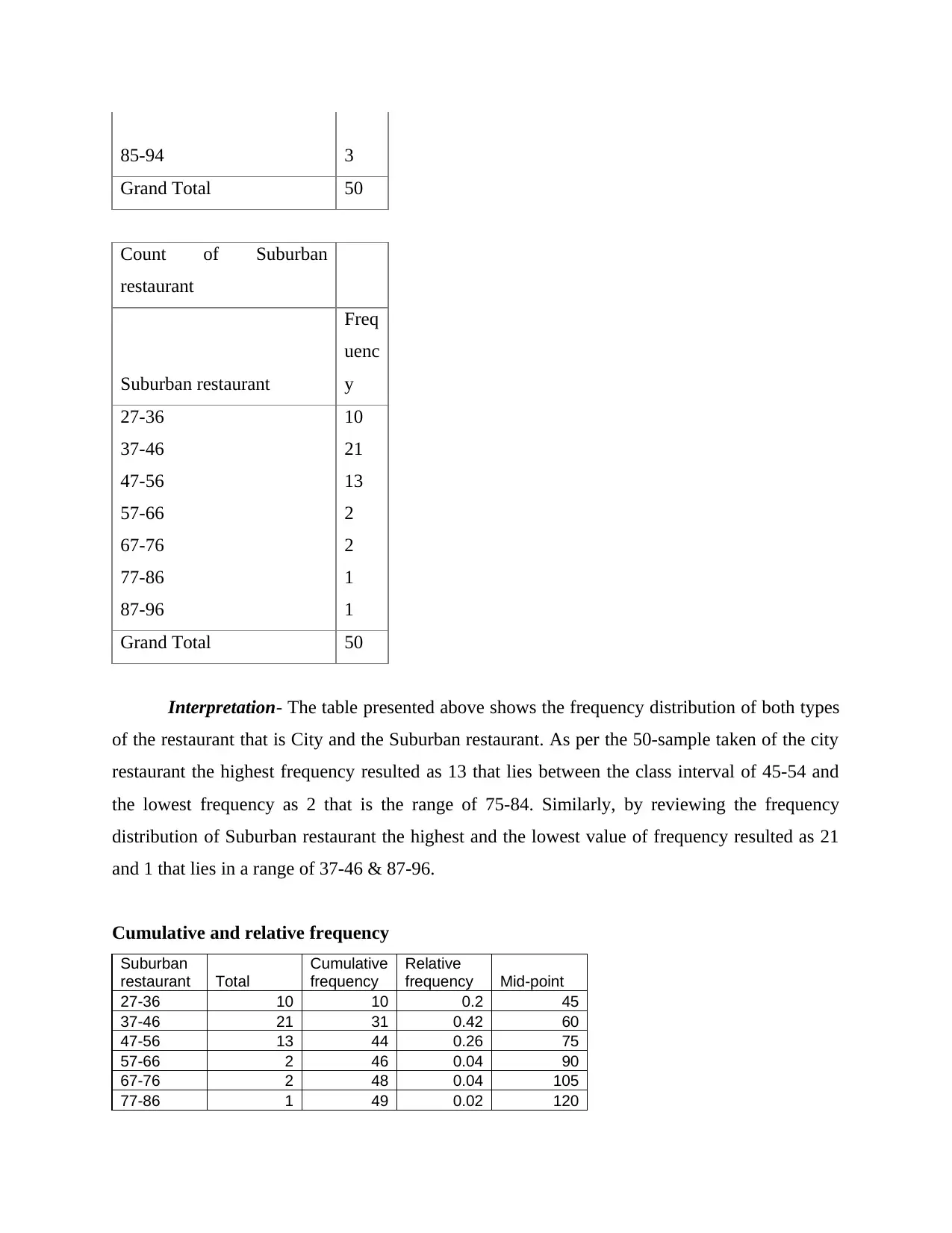
Count of Suburban
restaurant
Suburban restaurant
Freq
uenc
y
27-36 10
37-46 21
47-56 13
57-66 2
67-76 2
77-86 1
87-96 1
Grand Total 50
Interpretation- The table presented above shows the frequency distribution of both types
of the restaurant that is City and the Suburban restaurant. As per the 50-sample taken of the city
restaurant the highest frequency resulted as 13 that lies between the class interval of 45-54 and
the lowest frequency as 2 that is the range of 75-84. Similarly, by reviewing the frequency
distribution of Suburban restaurant the highest and the lowest value of frequency resulted as 21
and 1 that lies in a range of 37-46 & 87-96.
Cumulative and relative frequency
Suburban
restaurant Total
Cumulative
frequency
Relative
frequency Mid-point
27-36 10 10 0.2 45
37-46 21 31 0.42 60
47-56 13 44 0.26 75
57-66 2 46 0.04 90
67-76 2 48 0.04 105
77-86 1 49 0.02 120

87-96 1 50 0.02 135
Grand
Total 50 100 1
City
restaurant Total
Cumulative
frequency Relative frequency
25-34 8 8 0.16 42
35-44 12 20 0.24 57
45-54 13 33 0.26 72
55-64 9 42 0.18 87
65-74 3 45 0.06 102
75-84 2 47 0.04 117
85-94 3 50 0.06 132
Grand
Total 50 100 1
c. On the basis of the raw data calculation of the mean, median and the mode
Mean- It refers to the mathematical average of the set of a two and more of the numbers.
The mean for given dataset could be computed in various ways with an inclusion of an arithmetic

mean that uses sum of a number in a particular series (George and Mallery, 2016). It is counted
as an indicator which could be used by the firm for the purpose of analysing its performance.
Median- It refers to the middle number or value that is sorted in an ascending form, list of
the numbers could be more descriptive of a specific data than an average. It is used as the
opposed to the value of mean within which the outliers are seen in a sequence that may skew
average values.
Mode- It means the number which appears several numbers of time in the dataset. A
number might be having one modal value and more than one modal value.
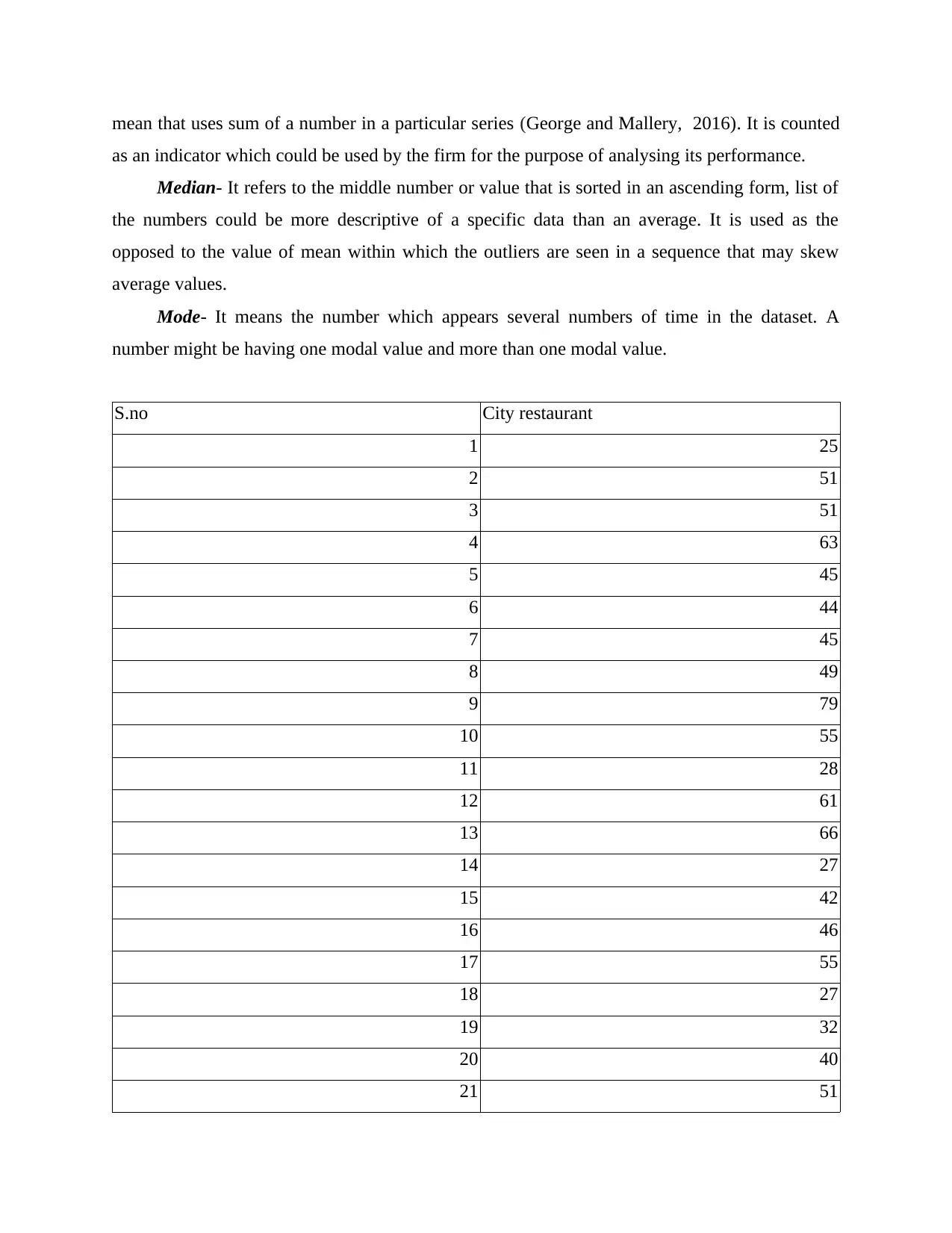
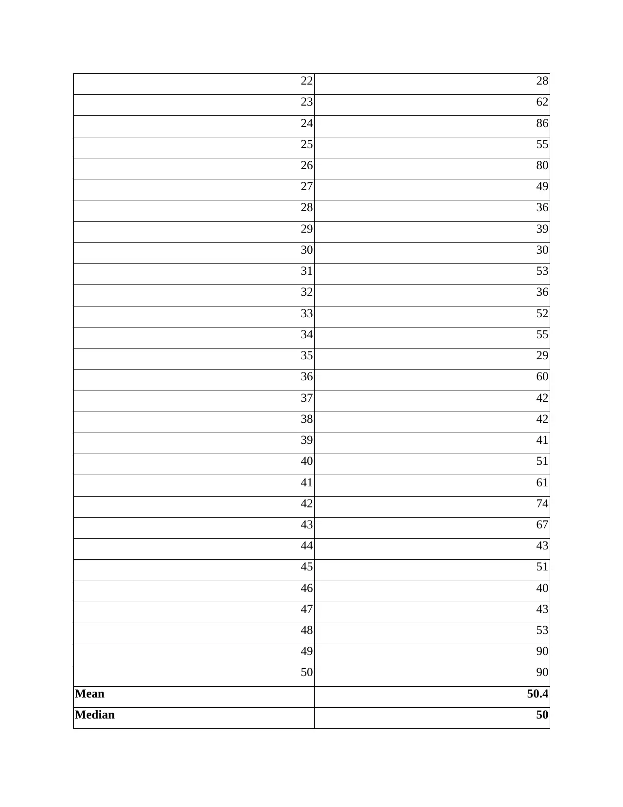
S.no City restaurant
1 25
2 51
3 51
4 63
5 45
6 44
7 45
8 49
9 79
10 55
11 28
12 61
13 66
14 27
15 42
16 46
17 55
18 27
19 32
20 40
21 51

22 28
23 62
24 86
25 55
26 80
27 49
28 36
29 39
30 30
31 53
32 36
33 52
34 55
35 29
36 60
37 42
38 42
39 41
40 51
41 61
42 74
43 67
44 43
45 51
46 40
47 43
48 53
49 90
50 90
Mean 50.4
Median 50

Mode 51
City restaurant
Mean 50.9183673
Median 51
Mode 51
Standard
Deviation 16.1230125
Range 63
Minimum 27
Maximum 90
Sum 2495
Count 49
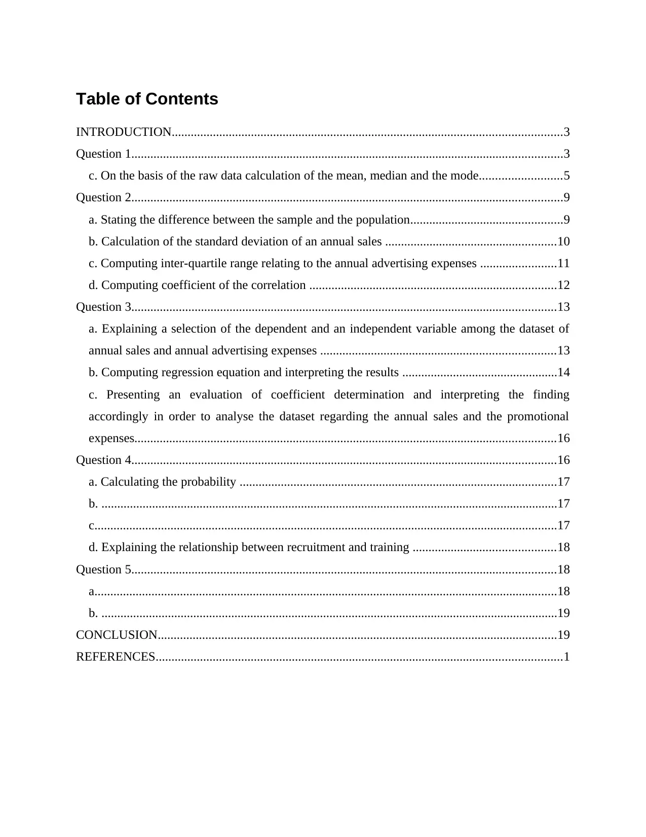
Interpretation- From the above analysis it has been analysed that the mean value of the
city restaurant resulted as 50.97 which is depicted as the average value of the dataset. It is
represented as the centre of a particular data and is determined by dividing the sum of the
frequency with that of the total number of an observation. The median value which is referred as
the mid value of the statistical data and is computed by applying the formula that is (n+1)/2
through which an observation that contains the value of median could be evaluated (Signorell,
and et.al., 2016). With respect to the data of city restaurant, the median value is presented as 51.
Moreover, the modal value of the city restaurant data accounted as 51 which reflects as the
number that is repeated frequently in the data which in turn also means that probability of an
individual in visiting the restaurant is said as 51 times.
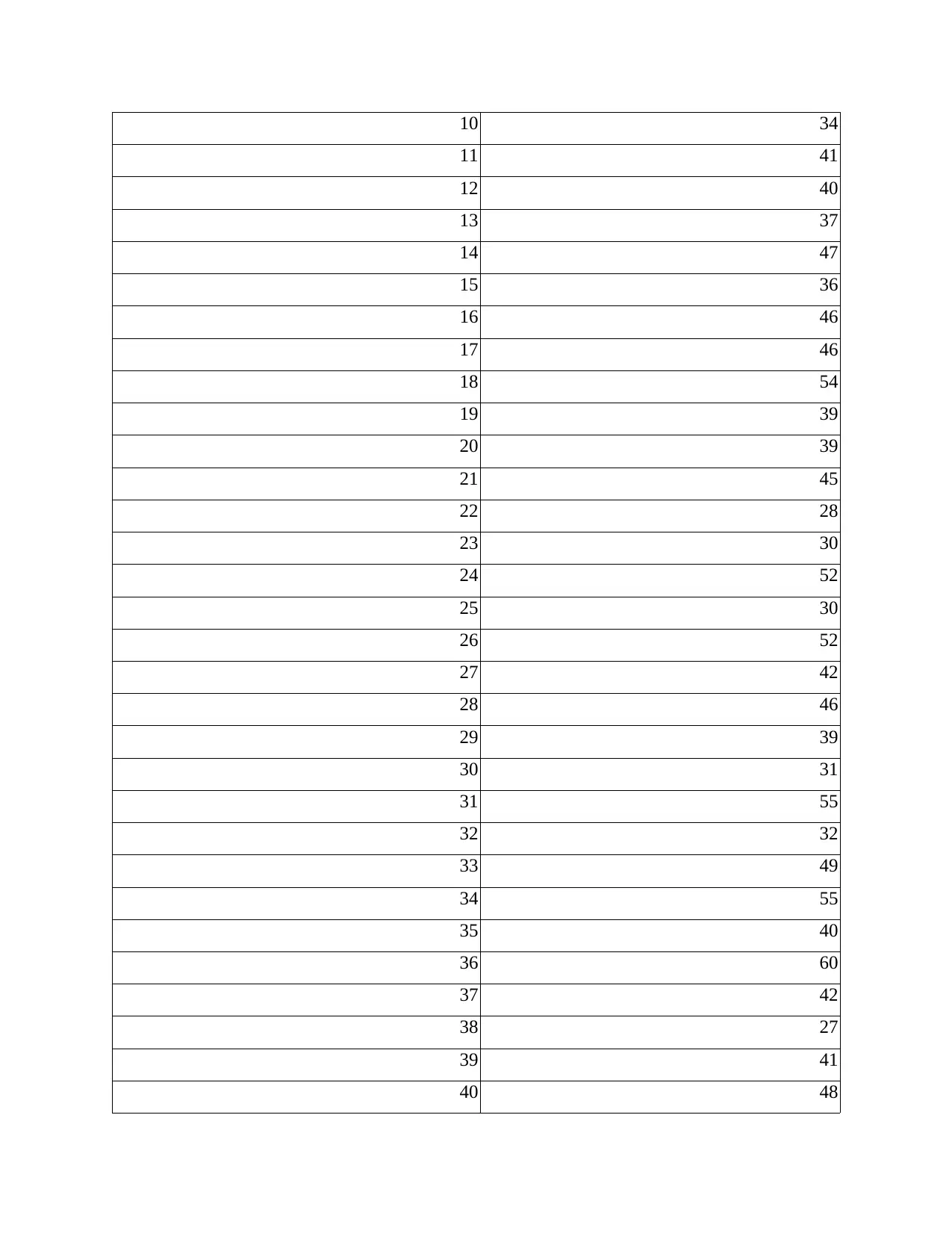
S.no. Suburban restaurant
1 33
2 31
3 46
4 50
5 56
6 49
7 46
8 38
9 46

10 34
11 41
12 40
13 37
14 47
15 36
16 46
17 46
18 54
19 39
20 39
21 45
22 28
23 30
24 52
25 30
26 52
27 42
28 46
29 39
30 31
31 55
32 32
33 49
34 55
35 40
36 60
37 42
38 27
39 41
40 48

41 61
42 70
43 74
44 43
45 51
46 40
47 43
48 53
49 80
50 89
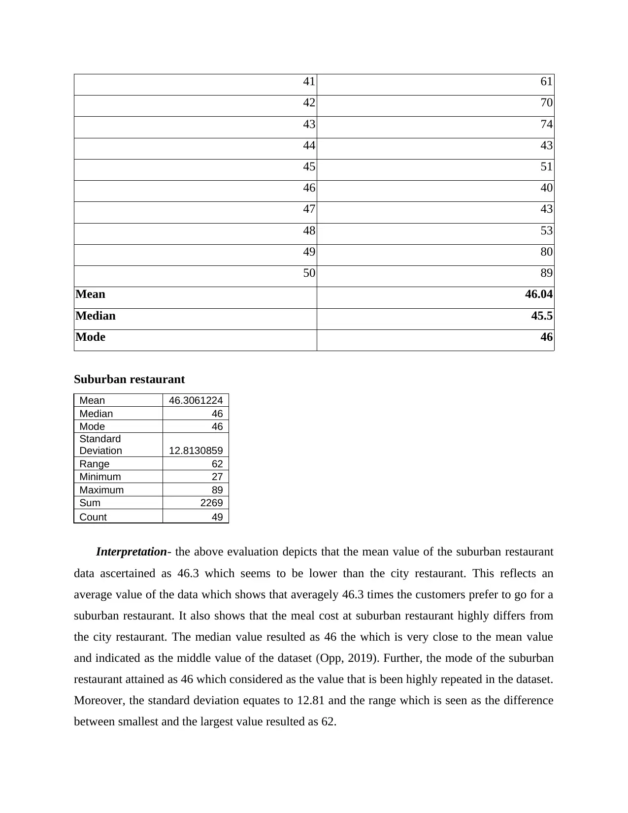
Mean 46.04
Median 45.5
Mode 46
Suburban restaurant
Mean 46.3061224
Median 46
Mode 46
Standard
Deviation 12.8130859
Range 62
Minimum 27
Maximum 89
Sum 2269
Count 49
Interpretation- the above evaluation depicts that the mean value of the suburban restaurant
data ascertained as 46.3 which seems to be lower than the city restaurant. This reflects an
average value of the data which shows that averagely 46.3 times the customers prefer to go for a
suburban restaurant. It also shows that the meal cost at suburban restaurant highly differs from
the city restaurant. The median value resulted as 46 the which is very close to the mean value
and indicated as the middle value of the dataset (Opp, 2019). Further, the mode of the suburban
restaurant attained as 46 which considered as the value that is been highly repeated in the dataset.
Moreover, the standard deviation equates to 12.81 and the range which is seen as the difference
between smallest and the largest value resulted as 62.

Question 2
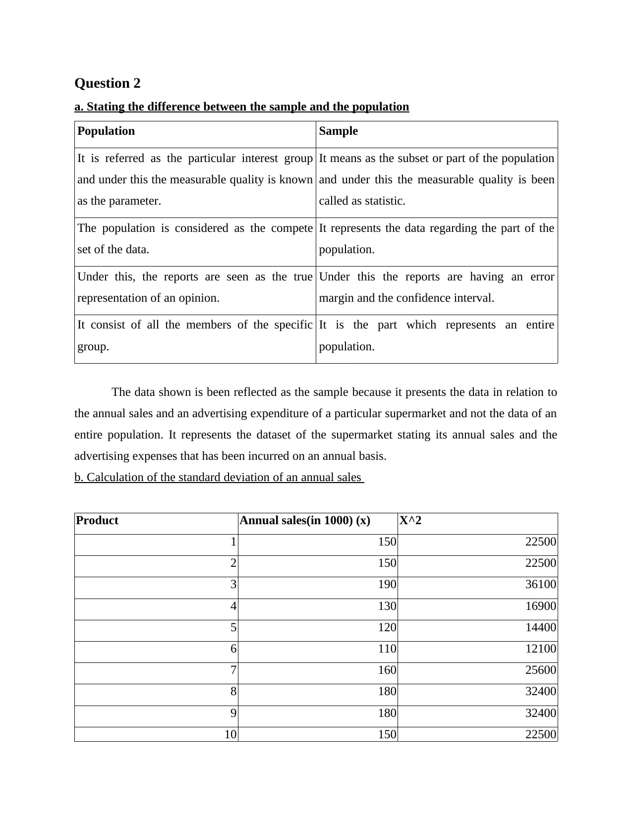
a. Stating the difference between the sample and the population
Population Sample
It is referred as the particular interest group
and under this the measurable quality is known
as the parameter.
It means as the subset or part of the population
and under this the measurable quality is been
called as statistic.
The population is considered as the compete
set of the data.
It represents the data regarding the part of the
population.
Under this, the reports are seen as the true
representation of an opinion.
Under this the reports are having an error
margin and the confidence interval.
It consist of all the members of the specific
group.
It is the part which represents an entire
population.
The data shown is been reflected as the sample because it presents the data in relation to
the annual sales and an advertising expenditure of a particular supermarket and not the data of an
entire population. It represents the dataset of the supermarket stating its annual sales and the
advertising expenses that has been incurred on an annual basis.
b. Calculation of the standard deviation of an annual sales
Product Annual sales(in 1000) (x) X^2
1 150 22500
2 150 22500
3 190 36100
4 130 16900
5 120 14400
6 110 12100
7 160 25600
8 180 32400
9 180 32400
10 150 22500

11 160 25600
12 140 19600
Total 1820 282600
Standard deviation= Square root of ∑x^2 / N – (∑x / n) ^ 2
= SQRT of (282600 / 12) – (1820 / 10) ^ 2
= SQRT of 23550 – 23002
= SQRT of 547.22
= 24.43
Interpretation- From the above assessment it has been identified that the standard
deviation of an annual sales of the supermarket evaluated as 24.43 which shows the dispersion
value from the mean. It is calculated by applying the formula and thereafter making the square
root of the value that is been attained from an equation or the formula. As the value of standard
deviation within the dataset is seen as large which clearly states that it is largely disperses from
the mean value or an average value and not depicted as close to the average or mean value.
c. Computing inter-quartile range relating to the annual advertising expenses
STEP 1 Arranging data in ascending order
Product Annual advertising expenditure
1 20
2 20
3 30
4 30
5 30
6 40
7 60
8 60
9 60
10 70
11 90

12 100
STEP
2 Making the mark in centre by dividing the data into two equal parts
20 20 30 30 30 40 I 60 60 60 70 90 100
STEP 3
Depicting the median value of upper and
lower half of the dataset
20
20
30
30
30
Q1 30
40
60
60
60
70
90
100
Q3 60
STEP 4
Subtracting the value of Q1 from the value
of Q3
Inter quartile range Q3-Q1
60-30
30

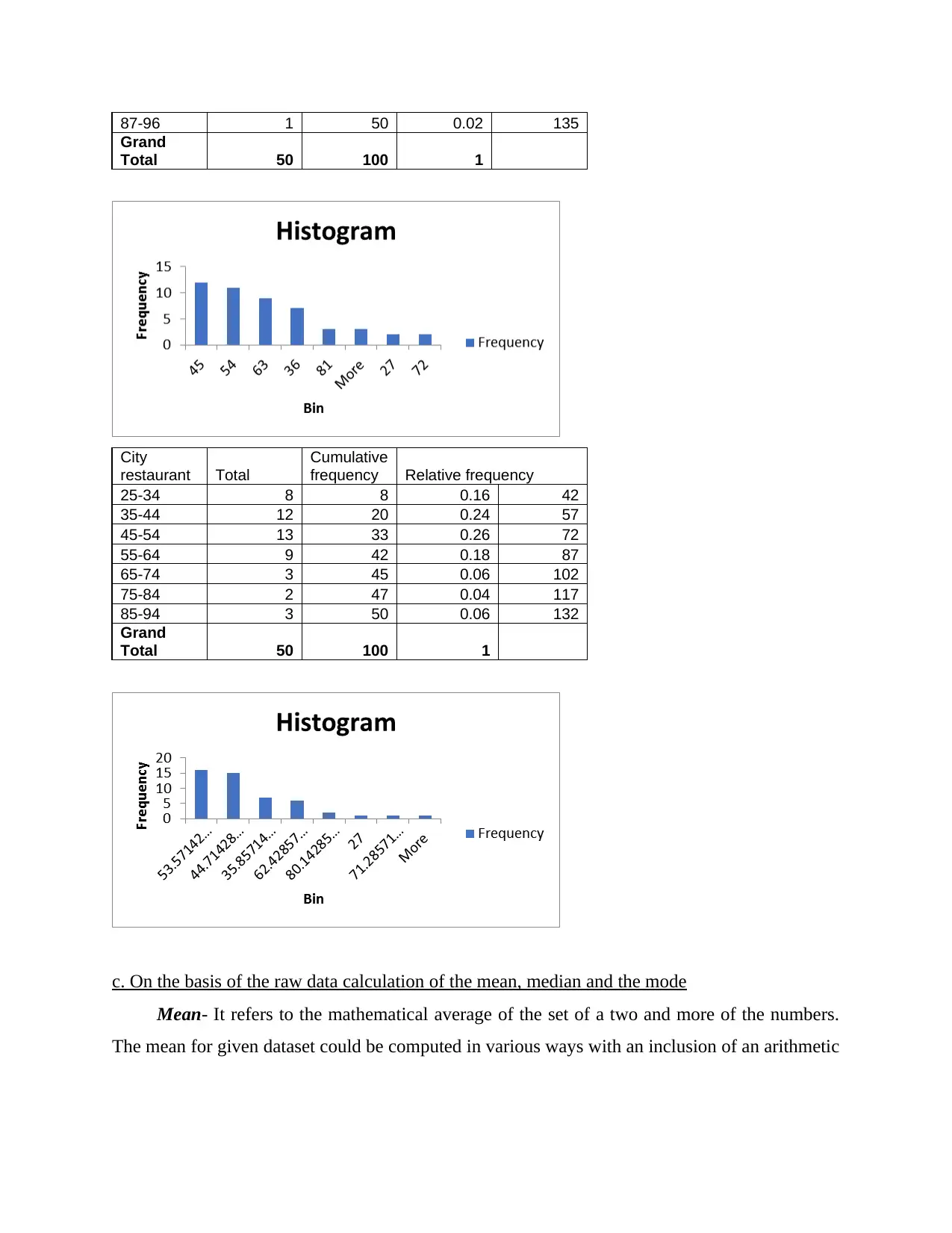
In the situation where computation of inter-quartile range is counted as most suitable than
standard deviation is where it requires an accurate evaluation of dataset. It is represented as the
middle of the data and is considered as most useful for the skewed of the data or the set of data
that contains an outliers. Inter-quartile is said as the resistant or the measure of the spread that is
not been easily influenced by such a low or the high values and provides for an accurate
determination of the data (Mak and et.al., 2017). An inter-quartile range of the data resulted as
30 by following an appropriate steps or sequence in respect to the even set of the observation.
IQR is found as the better measure than the standard deviation because it does not get affected by
the outliers. It is been reflected as the difference between upper and the lower values of quartiles
and describes middle of the values when it is been ordered from the lowest to the highest.
d. Computing coefficient of the correlation
Product Annual sales(in 1000)
Annual advertising
expenditure (in 1000)
1 150 60
2 150 60
3 190 100
4 130 30
5 120 20
6 110 20
7 160 30
8 180 70
9 180 90
10 150 40
11 160 30
12 140 60
Coefficient of correlation 0.80
Interpretation- The sign of correlation coefficient depicts a direction of a relationship
where positive coefficient shows that with an increase in the value of one variable, value of the

other variable seems to be increasing (Shaikh and Parulekar, 2018). By viewing the above data,
it has been seen that there is highly positive relationship present between annual sales and an
annual advertising expense which means that with change in the annual expenses relating to
advertising of the supermarket, its sales also changes with a higher proportion. As with more and
more expenses on the advertising , company could be able to attract larger customers that helps
in increasing the sales of the supermarket and this in turn also helps in increasing the profitability
of the company.
Question 3
a. Explaining a selection of the dependent and an independent variable among the dataset
of annual sales and annual advertising expenses
Product Annual sales(in 1000) (Y)
Annual advertising
expenditure (in 1000) (X)
1 150 60
2 150 60
3 190 100
4 130 30
5 120 20
6 110 20
7 160 30
8 180 70
9 180 90
10 150 40
11 160 30
12 140 60
As there seen a positive relationship between annual sales and advertising expenditure, it
is represented that sales is highly dependent on the advertising expenditure. By making huge
investment in the advertising, company could be able to increase its sales as advertisement is
considered as the medium through which more and more customers can be attracted towards the
product by offering them with different sales promotional offers and providing them a unique

quality or feature of the product (Sikder and et.al., 2019). Therefore, under the study annual sales
is taken as the dependent variable and advertising expenditure as independent variable.
b. Computing regression equation and interpreting the results
Regression analysis- It is the powerful tool of statistics that examines relationship
between two or more than two variables of the particular interest study. It is used for determining
probable changes that occurred within one variable for a given amount of the change in the
another (Gelman and et.al., 2019). It depicts a degree to which a variable are seen as correlated
with each other depending on the regression line. It is the widely used technique in all types of
the scientific disciplines. In an economics, it plays a crucial role in measuring and anticipating a
relationship among different economic variables.
Regression Statistics
Multiple R 0.8033806592
R Square 0.6454204836
Adjusted R Square 0.609962532
Standard Error 15.2591136408
Observations 12
ANOVA
df SS MS F Significance F
Regression 1
4238.2611756
424
4238.2611756
424
18.202418745
3 0.0016462451
Residual 10
2328.4054910
243
232.84054910
24
Total 11
6566.6666666
667
Coefficie
nts
Standard
Error t Stat P-value
Lower
95%
Upper
95%
Lower
95.0%
Upper
95.0%
Intercept 114.4139 9.779780 11.69902 3.708313 92.62322 136.2046 92.62322 136.2046

38754 7496 90154
33278094
E-007 93018 482061 93018 482061
Annual
advertisin
g
expenditu
re (in
1000) (X)
0.732840
5491
0.171769
0608
4.266429
2734
0.001646
2451
0.350115
2313
1.115565
867
0.350115
2313
1.115565
867
RESIDUAL OUTPUT
Observation
Predicted Annual sales(in
1000) (Y) Residuals
1 158.3843717001 -8.3843717001
2 158.3843717001 -8.3843717001
3 187.6979936642 2.3020063358
4 136.399155227 -6.399155227
5 129.070749736 -9.070749736
6 129.070749736 -19.070749736
7 136.399155227 23.600844773
8 165.7127771911 14.2872228089
9 180.3695881732 -0.3695881732
10 143.7275607181 6.2724392819
11 136.399155227 23.600844773
12 158.3843717001 -18.3843717001

Interpretation- The above table shows a regression analysis value of R resulted as 0.80
which presents a strong relationship between annual sales and the advertising expenditure. This
shows that with increasing in an advertising expenditure, the sales of a supermarket also
increases. This in turn reflects a positive and direct relationship between annual sales and an
advertising expenditure. The significance value accounted as 0.001 which is lower than 0.05 that
means alternative hypotheses is accepted which states that there is a direct relationship in the
sales revenue and an expenses relating to advertising.
c. Presenting an evaluation of coefficient determination and interpreting the finding accordingly
in order to analyse the dataset regarding the annual sales and the promotional expenses
Coefficients- It is expressed as R square within which the MSS is considered as the
model sum of the squares that is counted as sum total of the squares of a prediction from a linear
regression reducing the value of mean for a specific variable (Hryhorenko and et.al., 2019). It is
the measure that analyse an ability of the model in predicting or in explaining resultant outcome
of the linear regression. It indicates proportion of variance within the dependent variable that is
been predicted by the linear regression and a predictor variable that is stated as an independent
variable.
R Square 0.6454204836
Adjusted R Square 0.609962532
10 20 30 40 50 60 70 80 90 100 110
0
100
200
Annual advertising expenditure (in 1000) (X) Line Fit
Plot
Column G Column Q
Annual advertising expenditure (in 1000) (X)
Annual sales(in 1000) (Y)

Interpretations- The table indicates that value of R square in respect of the annual sales
and advertising expenditure resulted as 0.64 which shows that with the change in the advertising
expenditure the sales revenue of the supermarket will be changing with doubled amount or a
greater proportion (Aggarwal and et.al., 2017). The value shows highly positive relationship
exist between annual sales & the advertising expenditure. This shows that the sales with be
changing with a greater value if an expenses in advertisement are been increasingly made by the
manager of the supermarket.
Question 4
Probability is defined as the measure of the likelihood that depicts an occurrence of the
event in the random experiment (Aidara, 2018). Probability is been quantified as the number
that lies between the value of 0 and 1 where 0 reflects impossibility and probability equated as 1
shows a certainty. Higher the probability of an event, more likely is an occurrence of that event
in the future.
a. Calculating the probability
Scientific training Grass roots training Total
Recruited from
Holmes students 18 72 90
External recruitment 35 12 47
Total 53 84
Probability of choosing of the player from the homes and the Grass roots training
Grass roots/total of the recruited students from
Holmes 72/90
Probability 0.8
Interpretation- From the above table it has been assessed that the probability relating to
selection of the recruited students from the Holmes and a Grass roots training is resulted as 0.8.

This means that there is a certainty for the Holmes students in getting chosen for the Grass roots
training.
b.
Probability of a selection of an external recruitment who is been involved in the scientific
training
External recruitment / total of the scientific
training 35/53
Probability 0.7
Interpretation- Referring to the above computation, probability of choosing an external
recruitment in the scientific training is seen as 0.7. This means that 0.7 is the certainty as it is
close to 1 for the external recruiting for getting a scientific training.
c.
Probability of selecting the Holmes students who are in scientific training
Recruited students belongs to Homes/ Scientific
training 18/53
Probability 0.3
Interpretation- The results shows that the probability for the Holmes student in getting
chosen for the scientific training is counted as 0.3 (Pitman, 2018). This means that there is less
chances for the Holmes students in getting the scientific training.
d. Explaining the relationship between recruitment and training
Scientific training
Grassroot
training Total
Holmes students 18 72 90
External
recruitment 35 12 47
Total 53 84 137
Scientific training
Grassroot
training Total
Holmes students 34.82 55.18 90
External
recruitment 18.18 28.82 47
Total 53 84 137

Scientific training
Grassroot
training Total
Holmes students 8.12 5.13 13.25
External
recruitment 15.56 9.81 25.37
Total 23.68 14.94 38.62
Chi square 38.62
Degree of freedom 1
Chi square 0
It has been stated that training is wholly independent with respect to recruitment because
training relates with range of the planned activities that assist an employee in developing skills,
knowledge and the attitude needed by an enterprise and the required work. However, recruiting
means an overall process of selecting, attracting, short listing and appointing of the candidates
for the job within an entity (Van Fraassen and Halpern, 2017). Training does not depicts any
dependency on the recruitment though both are considered as the internal human resource
management function. Recruitment deals with attracting the best talent in an organization and
training deals with enhancing the skills of an employees in order to bring versatility in the
organization.
Question 5
a.
Z test helps in ascertaining the mean of the populations that is evenly distributed i.e. the
distribution is normal. Normal distribution can be termed as that type of distribution under which
the real valued random variables are distributed equally and the curve is distributed in a bell
shaped manner.
Z test is normally applied only when the distribution of the sample is done normally i.e.
there are equal number of distribution on both the sides. However, it cannot be stated that the use
of Z test is exclusive to the application on normal distribution only because there are certain non-
normal distribution cases as well where the Z test can be made applicable (Dinur and Livni
Navon, 2017). When the z test is used in the case of non- normal distribution, the standard
normal table that is usually consulted for this test is not used and the sample test is twice when
the data is distributed in a non-normal way. In case the z test is applied in the data that is non-

normal, it is transformed into data sets of the z scores. Therefore, the distribution of the z scores
is similar to that of the original distribution i.e. for instance, if the data is distributed in a
positively skewed manner, than the z test will also show the results that are positively skewed
(Wang and et.al., 2017).
However, there is another constraint that the applicability of the z test is possible only
when the difference between the non-normal data is not too vast i.e. the variance is not at a vast
scale because in this scenario, the chances of using a z test becomes minimal because the results
hence generated will not be correct.
Therefore, in the current case, it can be adequately concluded that since the variance is
similar of the assistant and the manager, the z test can be applied and it will help in generating
correct or approximately correct results.
b.
Average 850000
X 900000
STDEV 270000
Z value 0.185185185
Probability 7%
Interpretation- It has been interpreted that out of total sample probability of investment by 30%
people is just 7%.
CONCLUSION
By summing up the above report it has been presented that application of the statistical
tools like frequency distribution, central tendency that includes mean, median and mode helps in
evaluating accurate and correct findings of the dataset. The results shows that the cost of the
meal of city and suburban restaurant differs to a great extent as with change in the area and the
crowd the cost of the meal also changes. From the study it has also been assessed that there is
positive and the strong relationship present between annual sales and the annual advertising
expenditure as with more and more advertisement the sales of the company increases. Moreover,
regression analysis and the coefficient of the correlation is the statistical technique which states
the relationship between the dependent and an independent variable. It also helps in measuring
the high or the low, positive or the negative relationship present among the variables so that
analysis and results are interpreted accordingly. Training is seen as highly independent with

resect to the recruitment because both are seen as the different function that is played by the
human resource in the business organization. Probability is the measure that enables in knowing
the actual possibility for an individual or thing fro getting selected on a random basis.

REFERENCES
Books and journals
Aggarwal, H.K., and et.al., 2017. Prevalence of depression, anxiety and insomnia in chronic
kidney disease patients and their co-relation with the demographic
variables. Prilozi. 38(2). pp.35-44.
Aidara, N., 2018. Introduction to probability and statistics.
Dinur, I. and Livni Navon, I., 2017. Exponentially small soundness for the direct product z-test.
In 32nd Computational Complexity Conference (CCC 2017). Schloss Dagstuhl-Leibniz-
Zentrum fuer Informatik.
Gelman, A., and et.al., 2019. R-squared for Bayesian regression models. The American
Statistician. 73(3). pp.307-309.
George, D. and Mallery, P., 2016. Descriptive statistics. In IBM SPSS Statistics 23 Step by
Step (pp. 126-134). Routledge.
Hryhorenko, and et.al., 2019. Dynamics of infectious and parasitogenic morbidity at the children
population in the rural districts and corelation with water factor. Wiadomosci lekarskie
(Warsaw, Poland: 1960). 72(5 cz 2). pp.1029-1032.
Liu, L. and et.al., 2018. Quantitative analysis of NAD synthesis-breakdown fluxes. Cell
metabolism. 27(5). pp.1067-1080.
Mak and et.al., 2017. Polygenic scores via penalized regression on summary statistics. Genetic
epidemiology. 41(6). pp.469-480.
Opp, K.D., 2019. The rationality of political protest: A comparative analysis of rational choice
theory. Routledge.
Pitman, E.J., 2018. Some basic theory for statistical inference: Monographs on applied
probability and statistics. Chapman and Hall/CRC.
Shaikh, A. and Parulekar, P., 2018. Co-relation between VC & 6 Minute Walk Test in Patients
with Impaired Lung Functions. Indian Journal of Physiotherapy & Occupational
Therapy. 12(1).
Signorell, and et.al., 2016. DescTools: Tools for descriptive statistics. R package version 0.99. 18.
Sikder, S.K., and et.al., 2019. Geospatial analysis of building structures in megacity Dhaka: The
use of spatial statistics for promoting data-driven decision-MAKING. Journal of
Geovisualization and Spatial Analysis. 3(1). p.7.
1

Van Fraassen, B.C. and Halpern, J.Y., 2017. Updating probability: tracking statistics as
criterion. The British Journal for the Philosophy of Science. 68(3). pp.725-743.
Wang, T. and et.al., 2017. Dynamic low-resolution z test sizes. U.S. Patent Application
15/174,110.
2