EMAT30007 Applied Statistics: Linear Models for Sugar Consumption

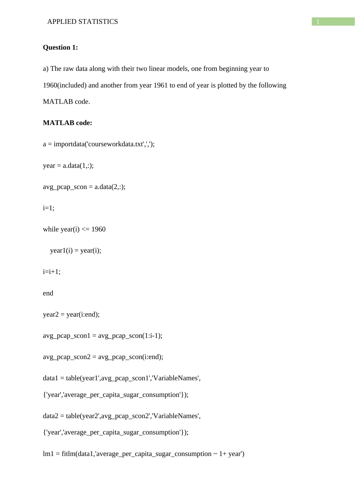
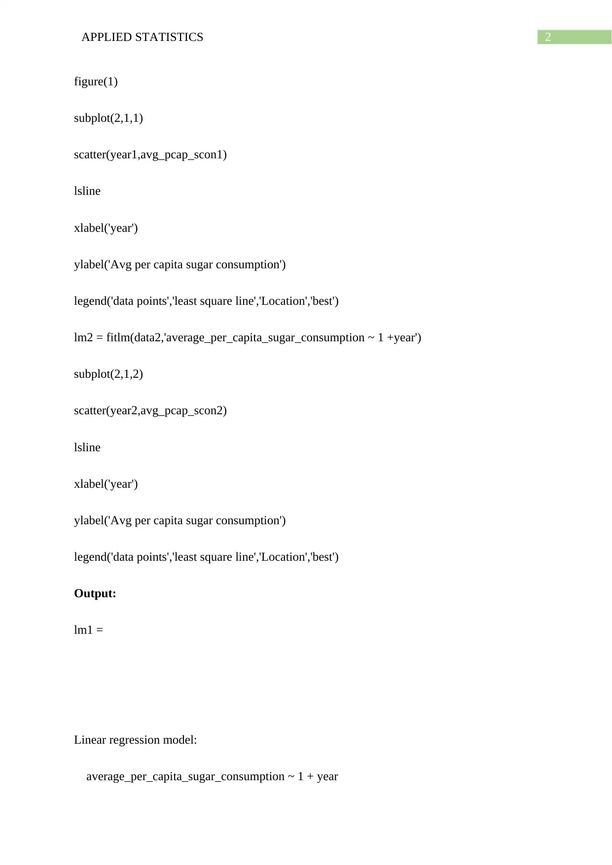
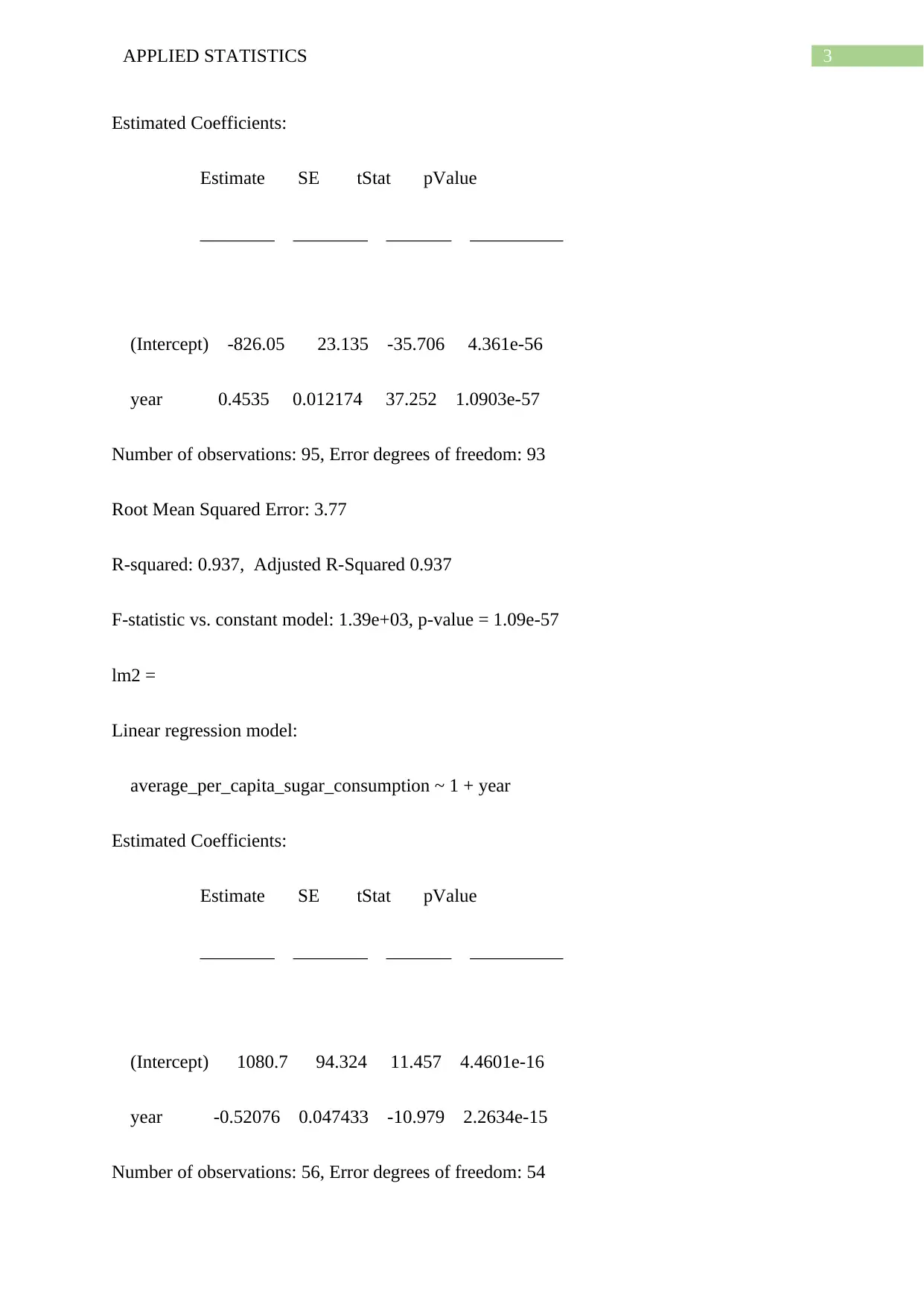
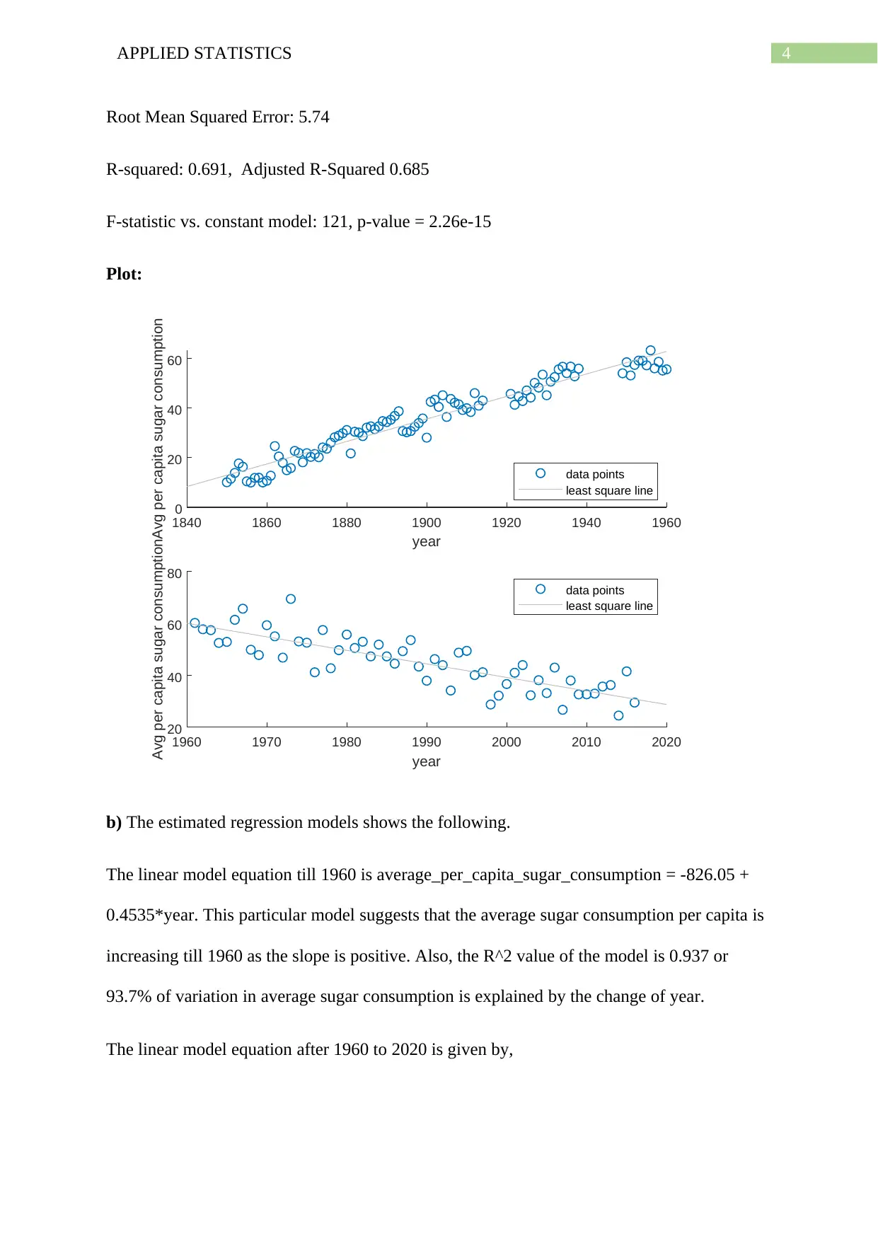
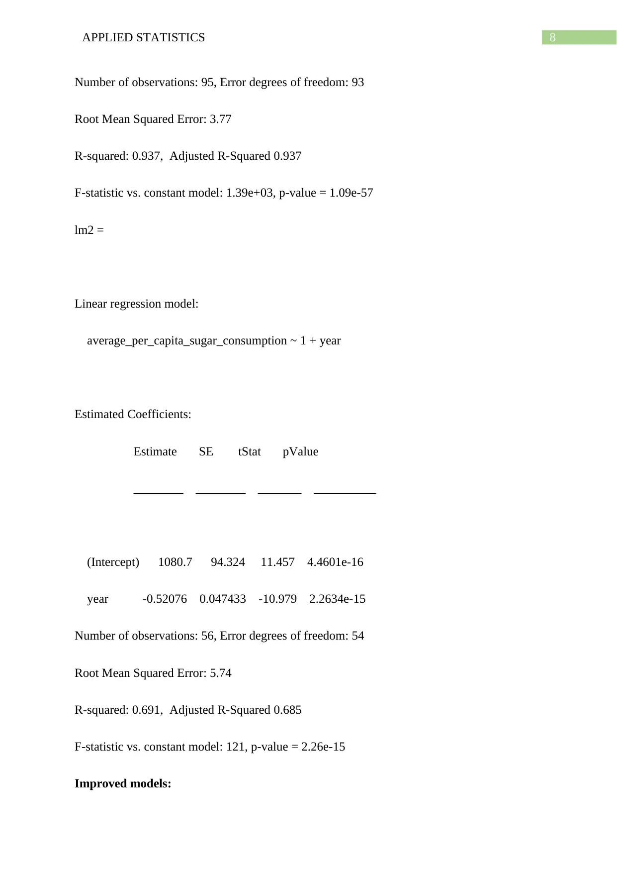
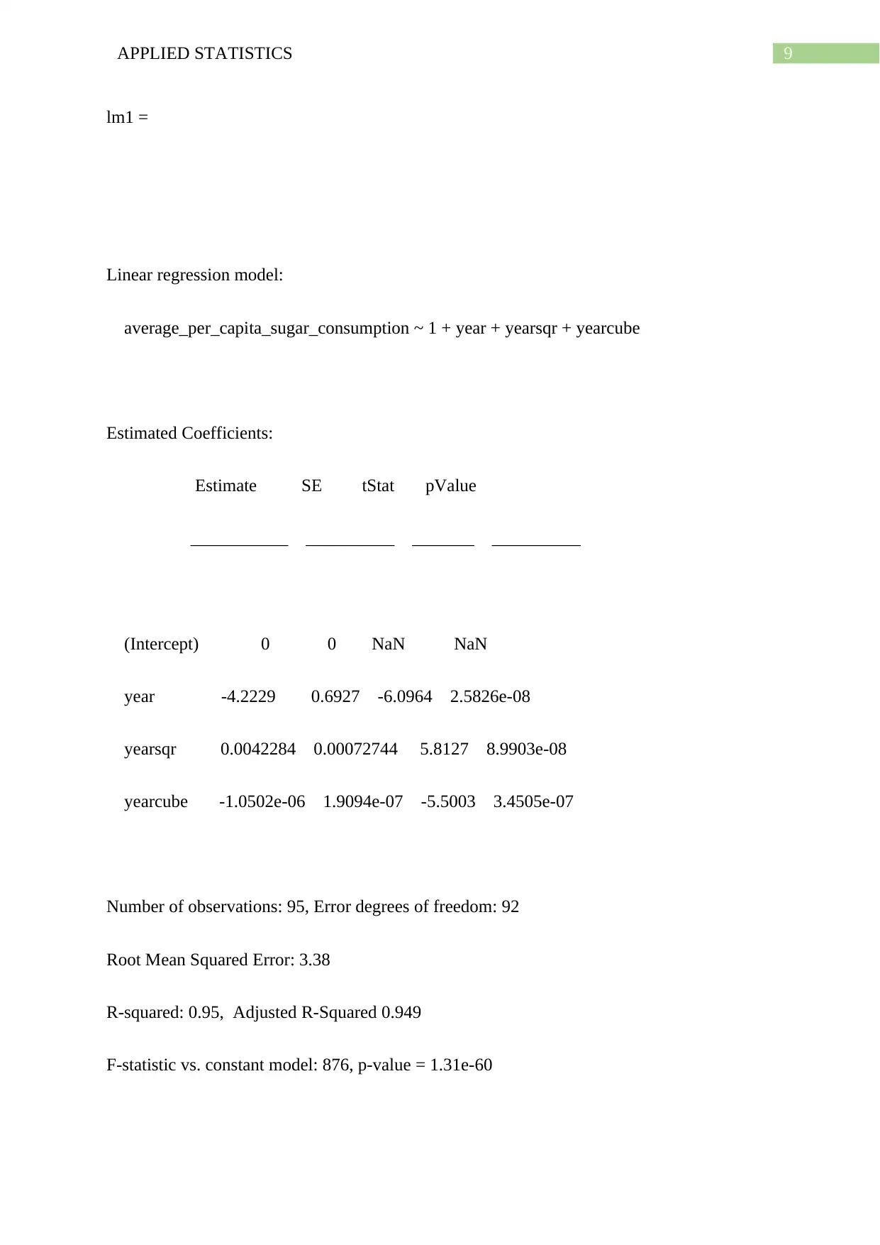
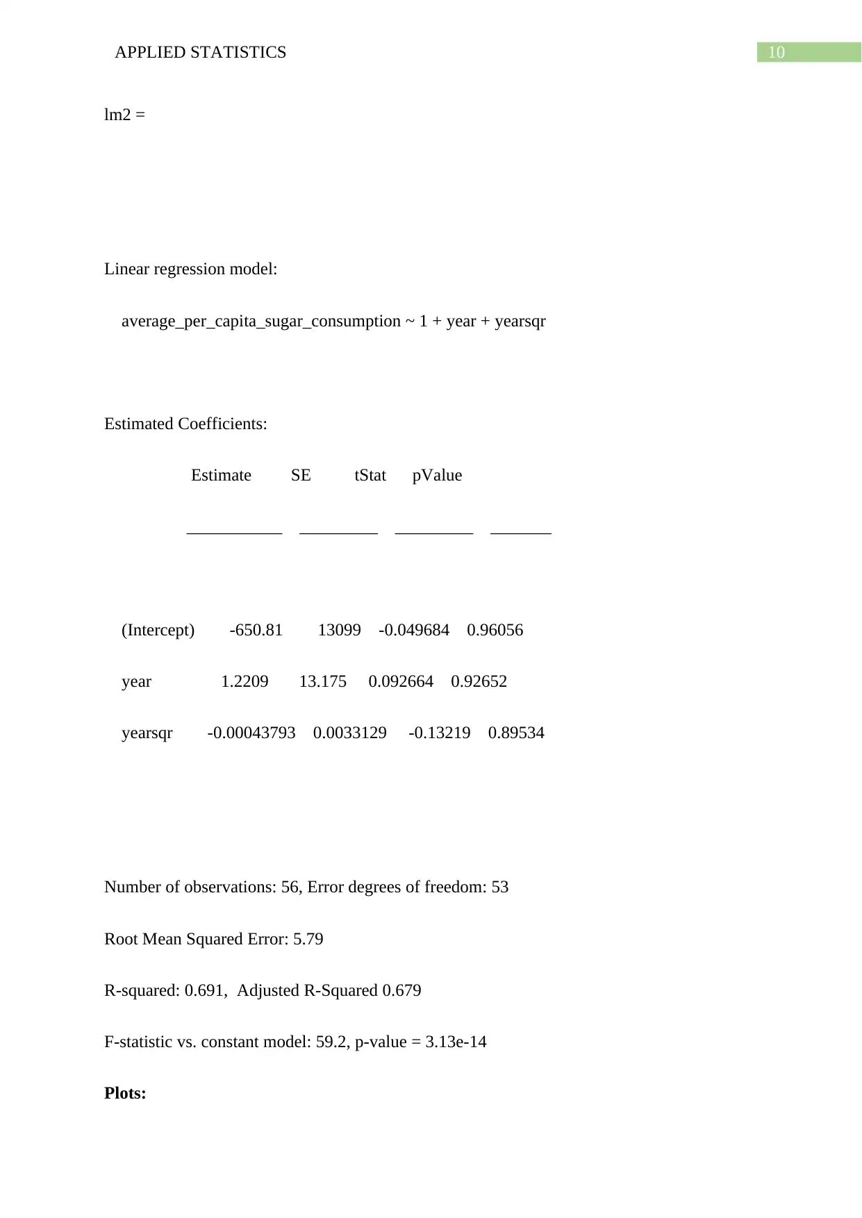
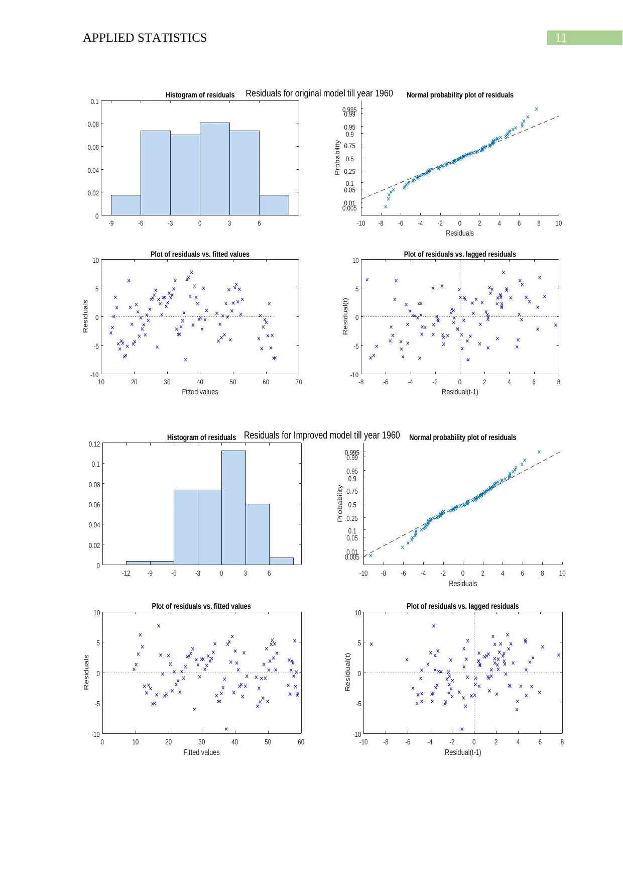
This document presents a comprehensive solution to an applied statistics assignment, focusing on the analysis of sugar consumption data using linear models. The assignment utilizes MATLAB to build and evaluate various linear regression models. The analysis begins by plotting raw data and fitting linear models to different time periods, examining the equations, R-squared values, and interpretations of the models. The solution then proceeds to improve the models by incorporating quadratic and cubic terms, performing residual analysis to assess model fit and identify areas for improvement. The predicted values for sugar consumption are calculated using the improved models, and the results are compared to historical evidence. Furthermore, the assignment explores the impact of including a quadratic term in a single linear model and compares the results to the previous models. The solution also covers the model parameters, residual plots, and interpretations of the results. Finally, the assignment incorporates Bayesian modeling to the data and examines the impact of prior distributions on the model's parameters.

Running head: APPLIED STATISTICS
APPLIED STATISTICS
Name of the Student
Name of the University
Author Note

1APPLIED STATISTICS
Question 1:
a) The raw data along with their two linear models, one from beginning year to
1960(included) and another from year 1961 to end of year is plotted by the following
MATLAB code.
MATLAB code:
a = importdata('courseworkdata.txt',',');
year = a.data(1,:);
avg_pcap_scon = a.data(2,:);
i=1;
while year(i) <= 1960
year1(i) = year(i);
i=i+1;
end
year2 = year(i:end);
avg_pcap_scon1 = avg_pcap_scon(1:i-1);
avg_pcap_scon2 = avg_pcap_scon(i:end);
data1 = table(year1',avg_pcap_scon1','VariableNames',
{'year','average_per_capita_sugar_consumption'});
data2 = table(year2',avg_pcap_scon2','VariableNames',
{'year','average_per_capita_sugar_consumption'});
lm1 = fitlm(data1,'average_per_capita_sugar_consumption ~ 1+ year')

2APPLIED STATISTICS
figure(1)
subplot(2,1,1)
scatter(year1,avg_pcap_scon1)
lsline
xlabel('year')
ylabel('Avg per capita sugar consumption')
legend('data points','least square line','Location','best')
lm2 = fitlm(data2,'average_per_capita_sugar_consumption ~ 1 +year')
subplot(2,1,2)
scatter(year2,avg_pcap_scon2)
lsline
xlabel('year')
ylabel('Avg per capita sugar consumption')
legend('data points','least square line','Location','best')
Output:
lm1 =
Linear regression model:
average_per_capita_sugar_consumption ~ 1 + year

3APPLIED STATISTICS
Estimated Coefficients:
Estimate SE tStat pValue
________ ________ _______ __________
(Intercept) -826.05 23.135 -35.706 4.361e-56
year 0.4535 0.012174 37.252 1.0903e-57
Number of observations: 95, Error degrees of freedom: 93
Root Mean Squared Error: 3.77
R-squared: 0.937, Adjusted R-Squared 0.937
F-statistic vs. constant model: 1.39e+03, p-value = 1.09e-57
lm2 =
Linear regression model:
average_per_capita_sugar_consumption ~ 1 + year
Estimated Coefficients:
Estimate SE tStat pValue
________ ________ _______ __________
(Intercept) 1080.7 94.324 11.457 4.4601e-16
year -0.52076 0.047433 -10.979 2.2634e-15
Number of observations: 56, Error degrees of freedom: 54

4APPLIED STATISTICS
Root Mean Squared Error: 5.74
R-squared: 0.691, Adjusted R-Squared 0.685
F-statistic vs. constant model: 121, p-value = 2.26e-15
Plot:
1840 1860 1880 1900 1920 1940 1960
year
0
20
40
60
Avg per capita sugar consumption
data points
least square line
1960 1970 1980 1990 2000 2010 2020
year
20
40
60
80
Avg per capita sugar consumption
data points
least square line
b) The estimated regression models shows the following.
The linear model equation till 1960 is average_per_capita_sugar_consumption = -826.05 +
0.4535*year. This particular model suggests that the average sugar consumption per capita is
increasing till 1960 as the slope is positive. Also, the R^2 value of the model is 0.937 or
93.7% of variation in average sugar consumption is explained by the change of year.
The linear model equation after 1960 to 2020 is given by,

5APPLIED STATISTICS
average_per_capita_sugar_consumption = 1080.7 -0.52076*year. Thus the model shows that
the average per capita consumption of sugar is decreasing after 1960 as the slope is negative.
The R^2 of the model is 0.691 or 69.1% of variation in the average per capita consumption of
the sugar is explained by the change in year.
c)
The model checking is performed where the models are improved with change in the
predictor variables. The improved models and the previous models are compared by the
residual plots.
MATLAB code:
%% Improved models
data1 = table(year1',(year1.^2)',(year1.^3)',avg_pcap_scon1','VariableNames',
{'year','yearsqr','yearcube','average_per_capita_sugar_consumption'});
data2 = table(year2',(year2.^2)',avg_pcap_scon2','VariableNames',
{'year','yearsqr','average_per_capita_sugar_consumption'});
lm1 = fitlm(data1,'average_per_capita_sugar_consumption ~ 1+ year + yearsqr + yearcube')
lm2 = fitlm(data2,'average_per_capita_sugar_consumption ~ 1 +year + yearsqr')
figure(4)
suptitle('Residuals for Improved model till year 1960')
subplot(2,2,1)

6APPLIED STATISTICS
plotResiduals(lm1)
% Q-Q plot for check normality
subplot(2,2,2)
plotResiduals(lm1,'probability')
% residuals versus fitted values
subplot(2,2,3)
plotResiduals(lm1,'fitted')
% auto-correlation (via lagged residuals)
subplot(2,2,4)
plotResiduals(lm1,'lagged')
figure(5)
suptitle('Residuals for Improved model from year 1961')
subplot(2,2,1)
plotResiduals(lm2)
% Q-Q plot for check normality
subplot(2,2,2)
plotResiduals(lm2,'probability')

7APPLIED STATISTICS
% residuals versus fitted values
subplot(2,2,3)
plotResiduals(lm2,'fitted')
% auto-correlation (via lagged residuals)
subplot(2,2,4)
plotResiduals(lm2,'lagged')
Output:
Original models:
lm1 =
Linear regression model:
average_per_capita_sugar_consumption ~ 1 + year
Estimated Coefficients:
Estimate SE tStat pValue
________ ________ _______ __________
(Intercept) -826.05 23.135 -35.706 4.361e-56
year 0.4535 0.012174 37.252 1.0903e-57

8APPLIED STATISTICS
Number of observations: 95, Error degrees of freedom: 93
Root Mean Squared Error: 3.77
R-squared: 0.937, Adjusted R-Squared 0.937
F-statistic vs. constant model: 1.39e+03, p-value = 1.09e-57
lm2 =
Linear regression model:
average_per_capita_sugar_consumption ~ 1 + year
Estimated Coefficients:
Estimate SE tStat pValue
________ ________ _______ __________
(Intercept) 1080.7 94.324 11.457 4.4601e-16
year -0.52076 0.047433 -10.979 2.2634e-15
Number of observations: 56, Error degrees of freedom: 54
Root Mean Squared Error: 5.74
R-squared: 0.691, Adjusted R-Squared 0.685
F-statistic vs. constant model: 121, p-value = 2.26e-15
Improved models:

9APPLIED STATISTICS
lm1 =
Linear regression model:
average_per_capita_sugar_consumption ~ 1 + year + yearsqr + yearcube
Estimated Coefficients:
Estimate SE tStat pValue
___________ __________ _______ __________
(Intercept) 0 0 NaN NaN
year -4.2229 0.6927 -6.0964 2.5826e-08
yearsqr 0.0042284 0.00072744 5.8127 8.9903e-08
yearcube -1.0502e-06 1.9094e-07 -5.5003 3.4505e-07
Number of observations: 95, Error degrees of freedom: 92
Root Mean Squared Error: 3.38
R-squared: 0.95, Adjusted R-Squared 0.949
F-statistic vs. constant model: 876, p-value = 1.31e-60

10APPLIED STATISTICS
lm2 =
Linear regression model:
average_per_capita_sugar_consumption ~ 1 + year + yearsqr
Estimated Coefficients:
Estimate SE tStat pValue
___________ _________ _________ _______
(Intercept) -650.81 13099 -0.049684 0.96056
year 1.2209 13.175 0.092664 0.92652
yearsqr -0.00043793 0.0033129 -0.13219 0.89534
Number of observations: 56, Error degrees of freedom: 53
Root Mean Squared Error: 5.79
R-squared: 0.691, Adjusted R-Squared 0.679
F-statistic vs. constant model: 59.2, p-value = 3.13e-14
Plots:

11APPLIED STATISTICS
Residuals for original model till year 1960
-9 -6 -3 0 3 6
0
0.02
0.04
0.06
0.08
0.1 Histogram of residuals
-10 -8 -6 -4 -2 0 2 4 6 8 10
Residuals
0.005
0.01
0.05
0.1
0.25
0.5
0.75
0.9
0.95
0.99
0.995
Probability
Normal probability plot of residuals
10 20 30 40 50 60 70
Fitted values
-10
-5
0
5
10
Residuals
Plot of residuals vs. fitted values
-8 -6 -4 -2 0 2 4 6 8
Residual(t-1)
-10
-5
0
5
10
Residual(t)
Plot of residuals vs. lagged residuals
Residuals for Improved model till year 1960
-12 -9 -6 -3 0 3 6
0
0.02
0.04
0.06
0.08
0.1
0.12 Histogram of residuals
-10 -8 -6 -4 -2 0 2 4 6 8 10
Residuals
0.005
0.01
0.05
0.1
0.25
0.5
0.75
0.9
0.95
0.99
0.995
Probability
Normal probability plot of residuals
0 10 20 30 40 50 60
Fitted values
-10
-5
0
5
10
Residuals
Plot of residuals vs. fitted values
-10 -8 -6 -4 -2 0 2 4 6 8
Residual(t-1)
-10
-5
0
5
10
Residual(t)
Plot of residuals vs. lagged residuals