Applied Statistics 13 Assignment: Regression and Error Analysis

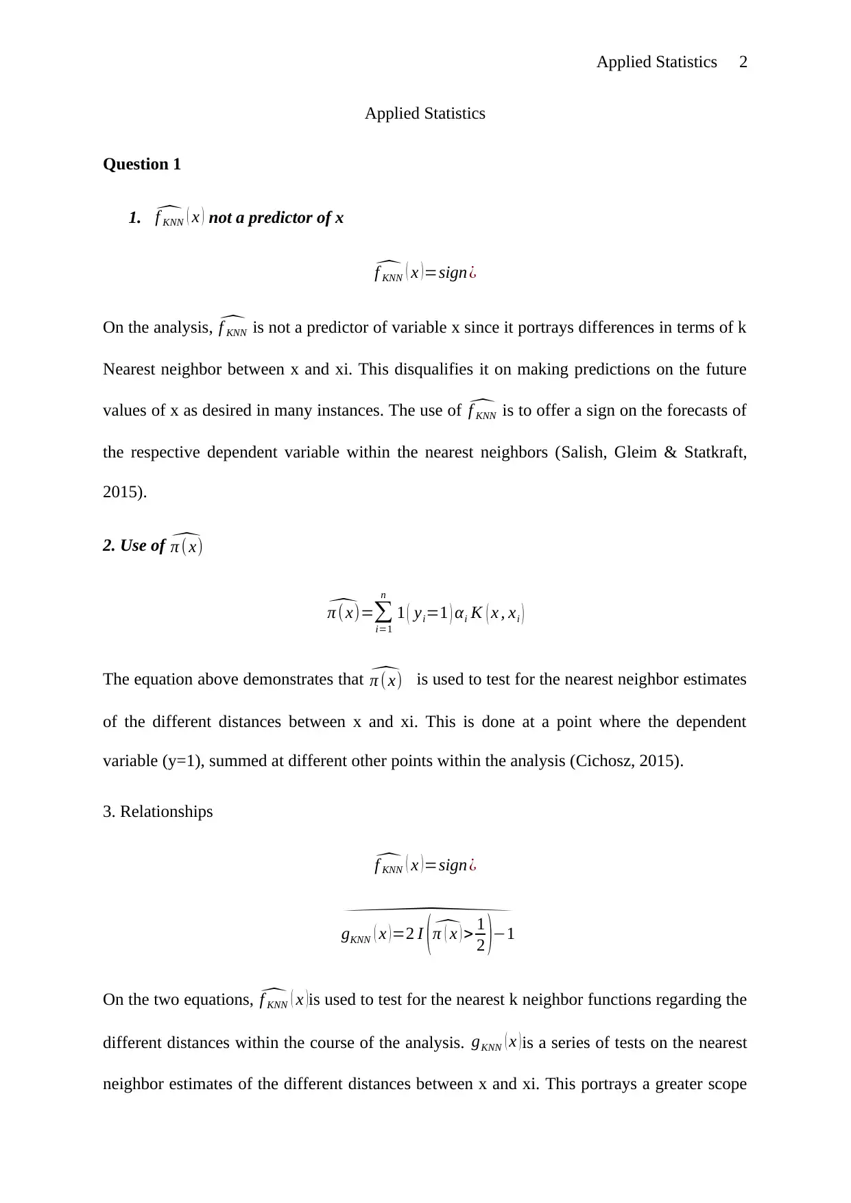
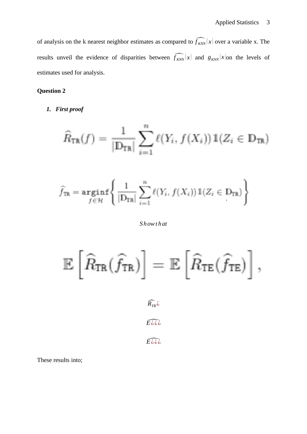
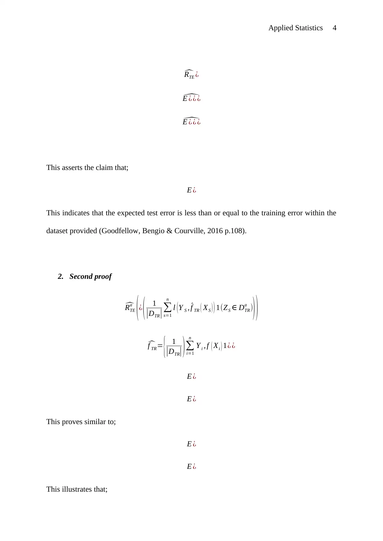
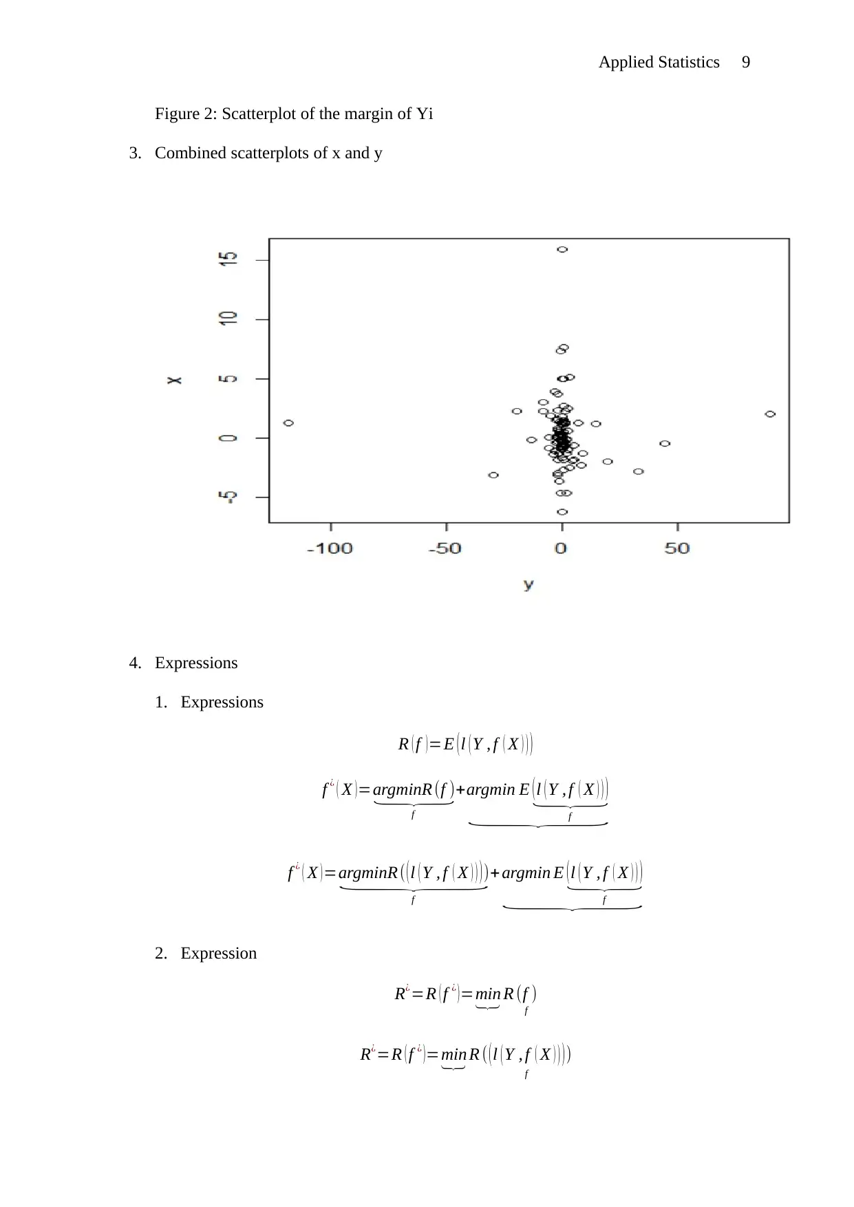
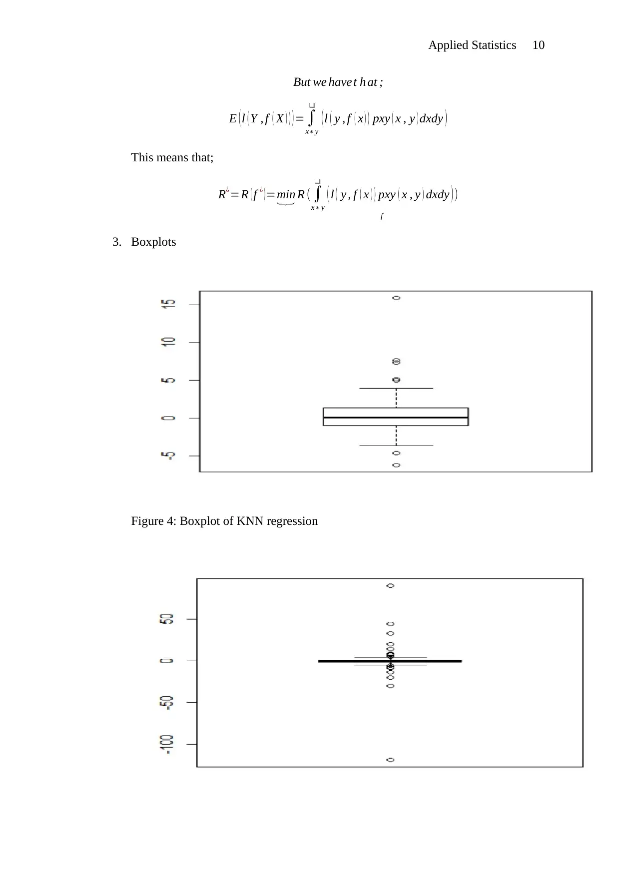
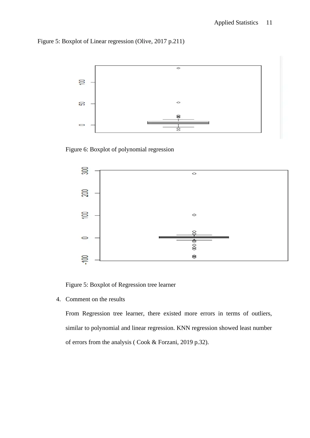
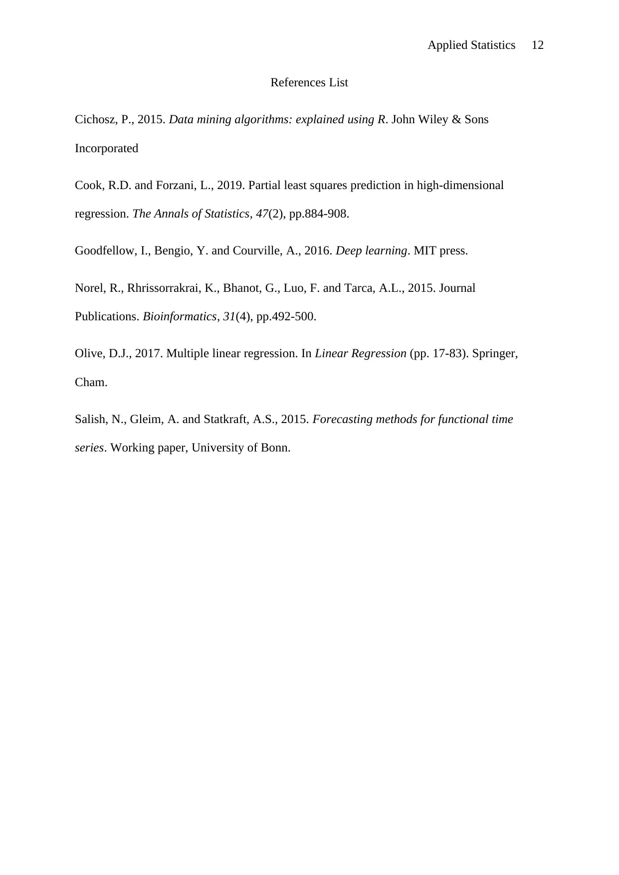
This document provides solutions to an Applied Statistics assignment. The assignment addresses three key questions. Question 1 focuses on the role of in the analysis, explaining its function and limitations as a predictor. Question 2 offers multiple proofs demonstrating the relationship between expected test error and training error. The proofs include mathematical derivations and comparisons. Question 3 involves the analysis of regression techniques. It includes scatterplots of marginal distributions, expressions, and boxplots comparing KNN regression, linear regression, polynomial regression, and regression tree learner. The analysis reveals error characteristics of each method, with the KNN regression showing the fewest outliers.

Applied Statistics 1
APPLIED STATISTICS
Student Name
Course
Professor
University
City (State)
Date

Applied Statistics 2
Applied Statistics
Question 1
1. ^f KNN ( x ) not a predictor of x
^f KNN ( x )=sign ¿
On the analysis, ^f KNN is not a predictor of variable x since it portrays differences in terms of k
Nearest neighbor between x and xi. This disqualifies it on making predictions on the future
values of x as desired in many instances. The use of ^f KNN is to offer a sign on the forecasts of
the respective dependent variable within the nearest neighbors (Salish, Gleim & Statkraft,
2015).
2. Use of ^π ( x)
^π ( x)=∑
i=1
n
1 ( yi=1 ) αi K ( x , xi )
The equation above demonstrates that ^π ( x) is used to test for the nearest neighbor estimates
of the different distances between x and xi. This is done at a point where the dependent
variable (y=1), summed at different other points within the analysis (Cichosz, 2015).
3. Relationships
^f KNN ( x )=sign ¿
^
gKNN ( x ) =2 I ( ^π ( x ) > 1
2 )−1
On the two equations, ^f KNN ( x )is used to test for the nearest k neighbor functions regarding the
different distances within the course of the analysis. gKNN ( x )is a series of tests on the nearest
neighbor estimates of the different distances between x and xi. This portrays a greater scope

Applied Statistics 3
of analysis on the k nearest neighbor estimates as compared to ^f KNN ( x ) over a variable x. The
results unveil the evidence of disparities between ^f KNN ( x ) and gKNN ( x )on the levels of
estimates used for analysis.
Question 2
1. First proof
S h ow t h at
^RTR ¿
^E ¿ ¿ ¿
^E ¿ ¿ ¿
These results into;

Applied Statistics 4
^RTE ¿
^E ¿ ¿ ¿
^E ¿ ¿ ¿
This asserts the claim that;
E ¿
This indicates that the expected test error is less than or equal to the training error within the
dataset provided (Goodfellow, Bengio & Courville, 2016 p.108).
2. Second proof
^RTE
a
( ¿ ( 1
|DTR| ∑
s=1
n
l ( Y S , ^f TR ( XS ) ) 1(ZS ∈ DTR
a )
) )
^f TR= { 1
|DTR| ) ∑
i=1
n
Y i , f ( Xi ) 1¿ ¿
E ¿
E ¿
This proves similar to;
E ¿
E ¿
This illustrates that;

Applied Statistics 5
E ¿
As required.
This indicates that the expected test error is less than or equal to the training error within the
dataset provided.
3. Third proof
¿ ¿
¿ ¿
¿ ¿
(Ra ¿¿ TE ( f TR ) )= 1
|DTR| ∑
s=1
n
l ( Y S , ^f TR ( XS ) ) 1 ( ZS ∈ DTR
a ) ¿ ¿
(Ra ¿¿ TE ( f TR ) )= 1
|DTR
2 |∑
s=1
n
l (Y S , ^f TR ( XS ) ) 1 ( ZS ∈ DTR
a ) ¿ ¿
This proves higher than the result from ¿ ¿, hence an indication that;
¿ ¿
This indicates that the expected test error is less than or equal to the training error within the
dataset provided.
4. Fourth proof
^
(R¿¿ TR¿)= 1
|DTR|∑
i=1
n
l (Y i , f ( Xi ) )1 (Zi ∈ DTR) ¿ ¿
( ^f TR ) ¿= { 1
|DTR| )∑
i=1
n
Y i , f ( Xi ) 1(¿ Zi ∈ DTR)¿

Applied Statistics 6
E ¿
E ¿
E ¿
¿
^f TR= { 1
|DTR| )∑
i=1
n
Y i , f ( Xi ) 1(¿ Zi ∈ DTR)¿
E ¿
E ¿
The analysis clearly demonstrates that;
E ¿
This indicates that the expected test error is less than or equal to the training error within the
dataset provided.
5. Graphical proof

Applied Statistics 7
From the graph, it is clear that the expected training error is less than the expected test
error from the figure above. This is in compliance with the expected results from the
analysis realized (Norel et al.,2015 p.496).
Question 3
1. E(Y|X)
E ( Y |X ) =E( 1
√ ( ( 2 π ) 9
2 π2 ) exp {−π2
18 [ y − π
2 x −3 π
4 cos ( π
2 ( 1+ x ) ] 2
}))
E ( Y |X ) = 1
√ ( ( 2 π ) 9
2 π 2 ) E (exp {−π2
18 [ y − π
2 x −3 π
4 cos ( π
2 ( 1+ x ) ] 2
}))
E ( Y |X ) = 1
√ ( ( 2 π ) 9
2 π 2 ) exp { −π 2
18 E [ y− π
2 x− 3 π
4 cos ( π
2 ( 1+x ) ]
2
})
2. Scatterplots of the marginal of x and y

Applied Statistics 8
Figure 1: Scatterplot of the margin of Xi

Applied Statistics 9
Figure 2: Scatterplot of the margin of Yi
3. Combined scatterplots of x and y
4. Expressions
1. Expressions
R ( f ) =E ( l ( Y , f ( X ) ) )
f ¿ ( X )=argminR (f )⏟
f
+argmin E (l ( Y , f ( X ) ) )⏟
f⏟
f ¿ ( X ) =argminR ( ( l ( Y , f ( X ) ) ) )⏟
f
+ argmin E ( l ( Y , f ( X ) ) )⏟
f⏟
2. Expression
R¿=R ( f ¿ )=min⏟ R (f )
f
R¿=R ( f ¿ ) =min⏟ R ( ( l ( Y , f ( X ) ) ) )
f

Applied Statistics 10
But we have t h at ;
E (l ( Y , f ( X ) ) )= ∫
x∗ y
❑
(l ( y , f ( x ) ) pxy ( x , y ) dxdy )
This means that;
R¿=R ( f ¿ ) =min⏟ R ( ∫
x∗ y
❑
( l ( y , f ( x ) ) pxy ( x , y ) dxdy ) )
f
3. Boxplots
Figure 4: Boxplot of KNN regression

Applied Statistics 11
Figure 5: Boxplot of Linear regression (Olive, 2017 p.211)
Figure 6: Boxplot of polynomial regression
Figure 5: Boxplot of Regression tree learner
4. Comment on the results
From Regression tree learner, there existed more errors in terms of outliers,
similar to polynomial and linear regression. KNN regression showed least number
of errors from the analysis ( Cook & Forzani, 2019 p.32).

Applied Statistics 12
References List
Cichosz, P., 2015. Data mining algorithms: explained using R. John Wiley & Sons
Incorporated
Cook, R.D. and Forzani, L., 2019. Partial least squares prediction in high-dimensional
regression. The Annals of Statistics, 47(2), pp.884-908.
Goodfellow, I., Bengio, Y. and Courville, A., 2016. Deep learning. MIT press.
Norel, R., Rhrissorrakrai, K., Bhanot, G., Luo, F. and Tarca, A.L., 2015. Journal
Publications. Bioinformatics, 31(4), pp.492-500.
Olive, D.J., 2017. Multiple linear regression. In Linear Regression (pp. 17-83). Springer,
Cham.
Salish, N., Gleim, A. and Statkraft, A.S., 2015. Forecasting methods for functional time
series. Working paper, University of Bonn.