Signals and Systems - Fourier Transform of Blood Flow Signal Analysis

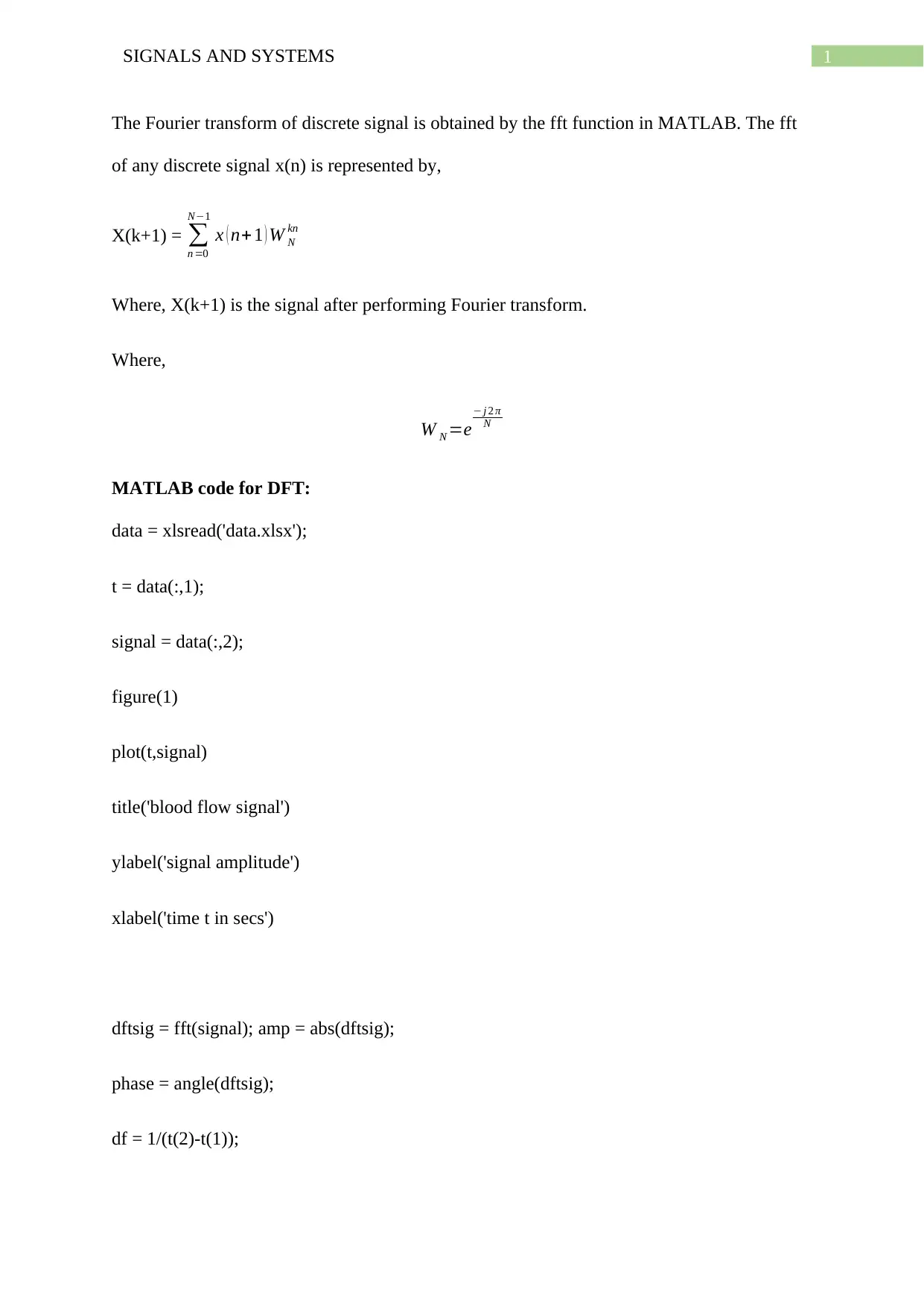
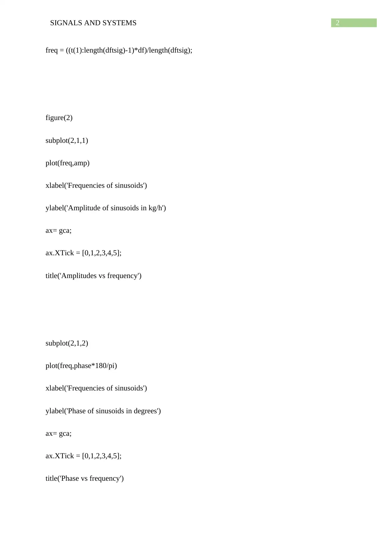
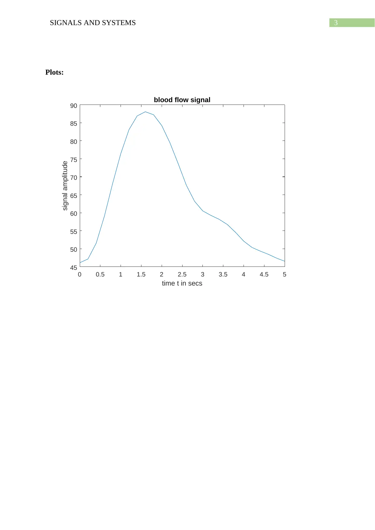
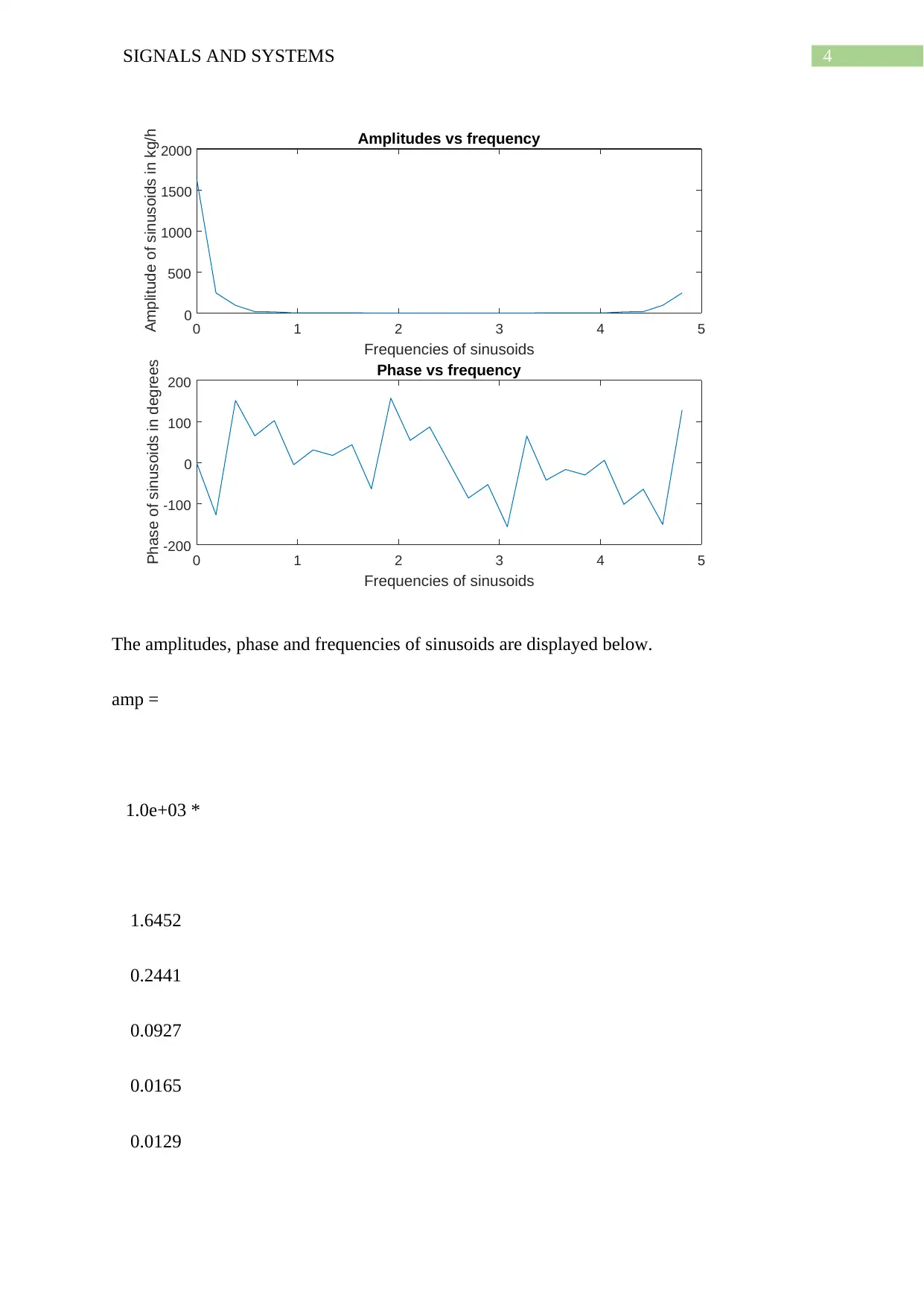
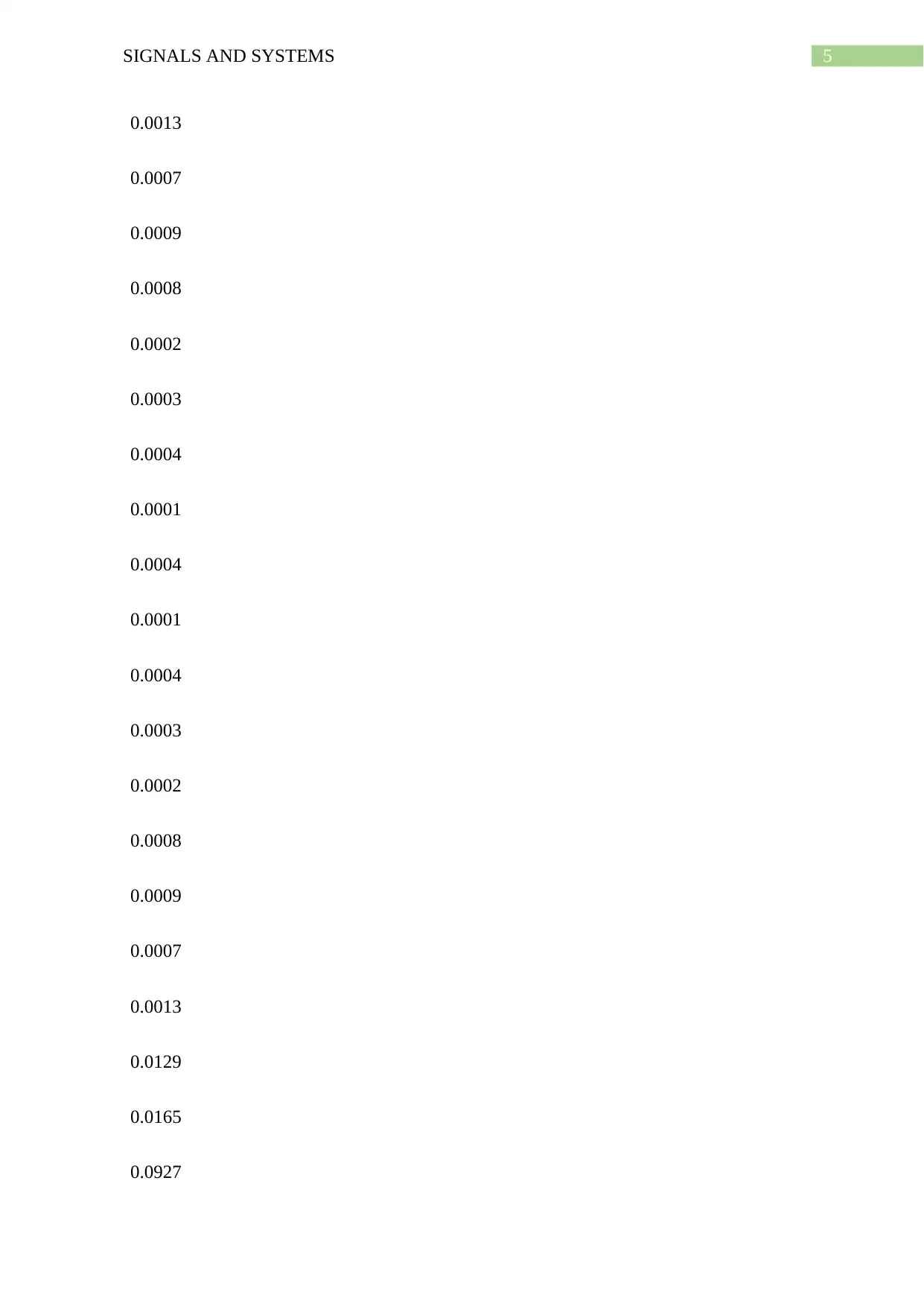
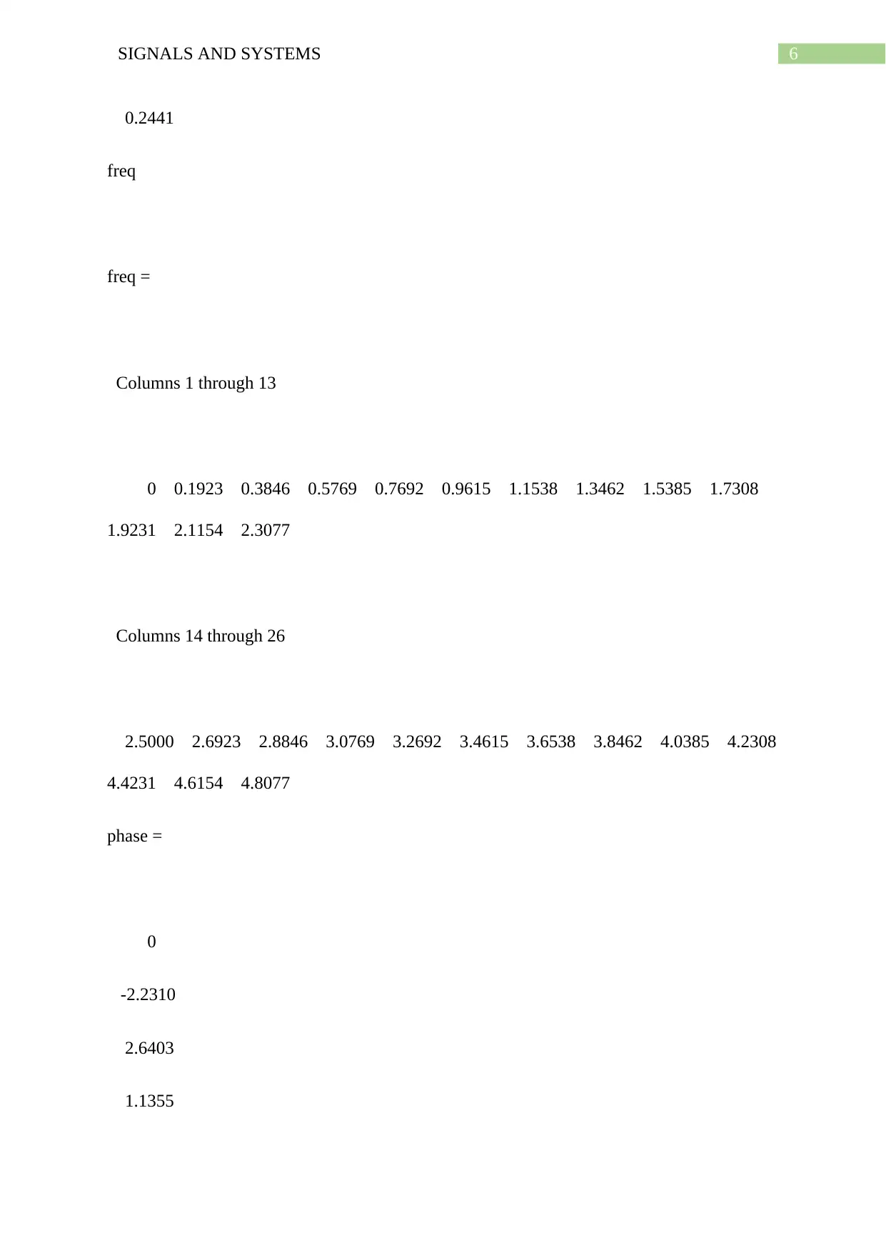
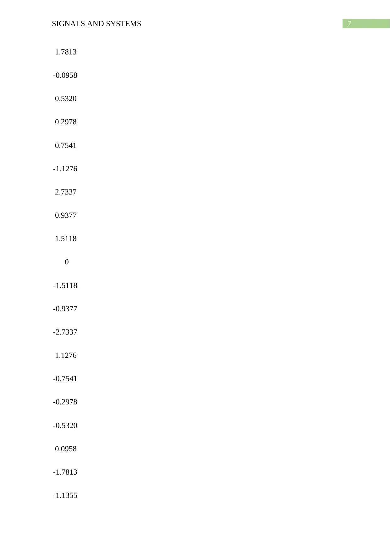
This assignment focuses on analyzing a blood flow signal using the Discrete Fourier Transform (DFT). The student implemented MATLAB code to read blood flow data, perform the DFT, and generate plots of the signal, its amplitude spectrum, and phase spectrum. The analysis includes calculations of frequencies, amplitudes, and phases of the sinusoidal components. The assignment provides the MATLAB code, the plots of the signal, and the resulting amplitude and phase values. The goal is to decompose the signal into a superposition of sine waves, which is crucial for repeatable analysis and mimicking the data accurately. The solution demonstrates the steps involved in transforming the signal from the time domain to the frequency domain, providing a detailed understanding of the frequency components present in the blood flow data, up to the 4th order.

Running head: SIGNALS AND SYSTEMS
SIGNALS AND SYSTEMS
Name of the Student
Name of the University
Author Note

1SIGNALS AND SYSTEMS
The Fourier transform of discrete signal is obtained by the fft function in MATLAB. The fft
of any discrete signal x(n) is represented by,
X(k+1) = ∑
n =0
N−1
x ( n+1 ) W N
kn
Where, X(k+1) is the signal after performing Fourier transform.
Where,
W N =e
− j 2 π
N
MATLAB code for DFT:
data = xlsread('data.xlsx');
t = data(:,1);
signal = data(:,2);
figure(1)
plot(t,signal)
title('blood flow signal')
ylabel('signal amplitude')
xlabel('time t in secs')
dftsig = fft(signal); amp = abs(dftsig);
phase = angle(dftsig);
df = 1/(t(2)-t(1));

2SIGNALS AND SYSTEMS
freq = ((t(1):length(dftsig)-1)*df)/length(dftsig);
figure(2)
subplot(2,1,1)
plot(freq,amp)
xlabel('Frequencies of sinusoids')
ylabel('Amplitude of sinusoids in kg/h')
ax= gca;
ax.XTick = [0,1,2,3,4,5];
title('Amplitudes vs frequency')
subplot(2,1,2)
plot(freq,phase*180/pi)
xlabel('Frequencies of sinusoids')
ylabel('Phase of sinusoids in degrees')
ax= gca;
ax.XTick = [0,1,2,3,4,5];
title('Phase vs frequency')

3SIGNALS AND SYSTEMS
Plots:
0 0.5 1 1.5 2 2.5 3 3.5 4 4.5 5
time t in secs
45
50
55
60
65
70
75
80
85
90
signal amplitude
blood flow signal

4SIGNALS AND SYSTEMS
0 1 2 3 4 5
Frequencies of sinusoids
0
500
1000
1500
2000
Amplitude of sinusoids in kg/h Amplitudes vs frequency
0 1 2 3 4 5
Frequencies of sinusoids
-200
-100
0
100
200
Phase of sinusoids in degrees
Phase vs frequency
The amplitudes, phase and frequencies of sinusoids are displayed below.
amp =
1.0e+03 *
1.6452
0.2441
0.0927
0.0165
0.0129

5SIGNALS AND SYSTEMS
0.0013
0.0007
0.0009
0.0008
0.0002
0.0003
0.0004
0.0001
0.0004
0.0001
0.0004
0.0003
0.0002
0.0008
0.0009
0.0007
0.0013
0.0129
0.0165
0.0927

6SIGNALS AND SYSTEMS
0.2441
freq
freq =
Columns 1 through 13
0 0.1923 0.3846 0.5769 0.7692 0.9615 1.1538 1.3462 1.5385 1.7308
1.9231 2.1154 2.3077
Columns 14 through 26
2.5000 2.6923 2.8846 3.0769 3.2692 3.4615 3.6538 3.8462 4.0385 4.2308
4.4231 4.6154 4.8077
phase =
0
-2.2310
2.6403
1.1355

7SIGNALS AND SYSTEMS
1.7813
-0.0958
0.5320
0.2978
0.7541
-1.1276
2.7337
0.9377
1.5118
0
-1.5118
-0.9377
-2.7337
1.1276
-0.7541
-0.2978
-0.5320
0.0958
-1.7813
-1.1355

8SIGNALS AND SYSTEMS
-2.6403
2.2310