Statistics and Probability Analysis Homework - Health Clubs
VerifiedAdded on 2023/01/05
|12
|1561
|77
Homework Assignment
AI Summary
This assignment presents a comprehensive statistical analysis of data related to California health and fitness clubs. It explores various statistical concepts, including confidence intervals, hypothesis testing, and regression analysis. The assignment covers topics such as calculating confidence intervals for population means, formulating and testing hypotheses about chest depth, analyzing the proportion of females, and examining relationships between waist and navel girths, and knee girths. The student utilizes both hand calculations and SPSS to derive statistical values, including p-values, t-statistics, and standard deviations, and discusses the implications of these findings. The assignment also delves into probability calculations, specifically the probability related to staff travel times, and explores the application of normal distributions. The student explains the reasoning behind differences observed in the calculations and provides interpretations of the results within the context of the provided data.
ASSESMENT
Paraphrase This Document
Need a fresh take? Get an instant paraphrase of this document with our AI Paraphraser
Contents
MAIN BODY..............................................................................................................................................3
Question 1...............................................................................................................................................3
Question 2...............................................................................................................................................5
Question 3...............................................................................................................................................6
Question 4...............................................................................................................................................8
Question 5.............................................................................................................................................11

MAIN BODY
Question 1
(a) 99% confidence interval-
99% Confidence Interval: 70 ± 1.66
(68.3 to 71.7)
"With 99% confidence the population mean is between 68.3 and 71.7, based on 60
samples."
Short Styles:
70 (99% CI 68.3 to 71.7)
70, 99% CI [68.3, 71.7]
Margin of Error: 1.66
(To more digits: 1.663)
Sample Size: 60
Sample Mean: 70
Standard Deviation: 5
Confidence Level: 99%
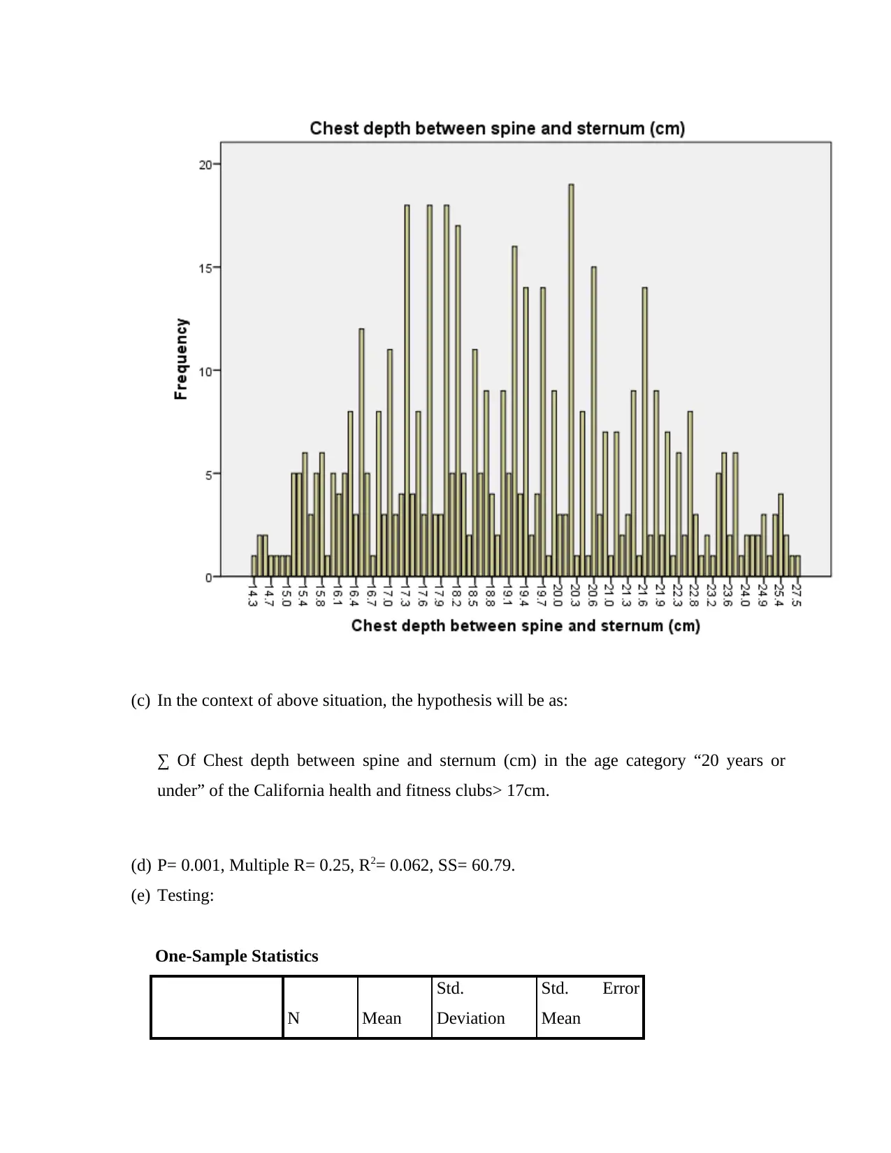
(b) Graph:
⊘ This is a preview!⊘
Do you want full access?
Subscribe today to unlock all pages.

Trusted by 1+ million students worldwide
(c) In the context of above situation, the hypothesis will be as:
∑ Of Chest depth between spine and sternum (cm) in the age category “20 years or
under” of the California health and fitness clubs> 17cm.
(d) P= 0.001, Multiple R= 0.25, R2= 0.062, SS= 60.79.
(e) Testing:
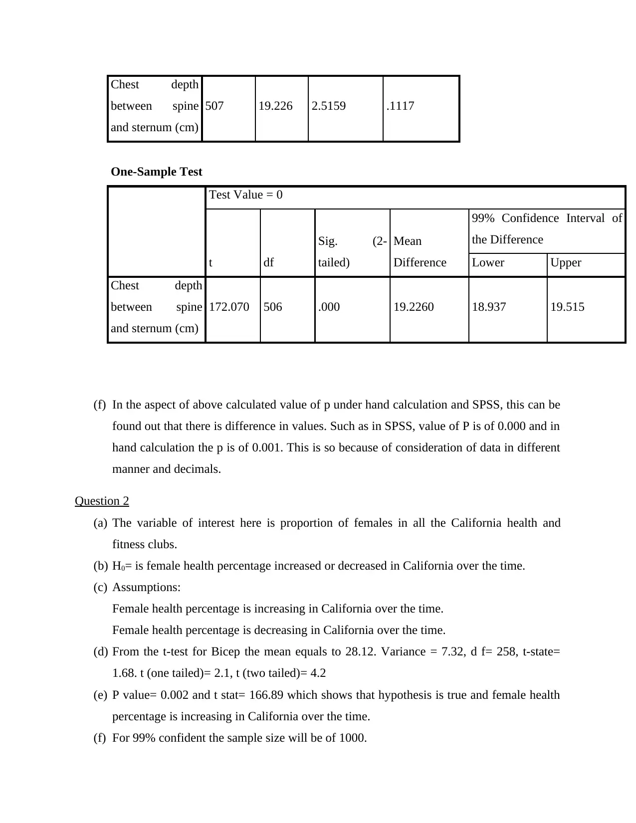
One-Sample Statistics
N Mean
Std.
Deviation
Std. Error
Mean
∑ Of Chest depth between spine and sternum (cm) in the age category “20 years or
under” of the California health and fitness clubs> 17cm.
(d) P= 0.001, Multiple R= 0.25, R2= 0.062, SS= 60.79.
(e) Testing:
One-Sample Statistics
N Mean
Std.
Deviation
Std. Error
Mean
Paraphrase This Document
Need a fresh take? Get an instant paraphrase of this document with our AI Paraphraser
Chest depth
between spine
and sternum (cm)
507 19.226 2.5159 .1117
One-Sample Test
Test Value = 0
t df
Sig. (2-
tailed)
Mean
Difference
99% Confidence Interval of
the Difference
Lower Upper
Chest depth
between spine
and sternum (cm)
172.070 506 .000 19.2260 18.937 19.515
(f) In the aspect of above calculated value of p under hand calculation and SPSS, this can be
found out that there is difference in values. Such as in SPSS, value of P is of 0.000 and in
hand calculation the p is of 0.001. This is so because of consideration of data in different
manner and decimals.
Question 2
(a) The variable of interest here is proportion of females in all the California health and
fitness clubs.
(b) H0= is female health percentage increased or decreased in California over the time.
(c) Assumptions:
Female health percentage is increasing in California over the time.
Female health percentage is decreasing in California over the time.
(d) From the t-test for Bicep the mean equals to 28.12. Variance = 7.32, d f= 258, t-state=
1.68. t (one tailed)= 2.1, t (two tailed)= 4.2
(e) P value= 0.002 and t stat= 166.89 which shows that hypothesis is true and female health
percentage is increasing in California over the time.
(f) For 99% confident the sample size will be of 1000.
between spine
and sternum (cm)
507 19.226 2.5159 .1117
One-Sample Test
Test Value = 0
t df
Sig. (2-
tailed)
Mean
Difference
99% Confidence Interval of
the Difference
Lower Upper
Chest depth
between spine
and sternum (cm)
172.070 506 .000 19.2260 18.937 19.515
(f) In the aspect of above calculated value of p under hand calculation and SPSS, this can be
found out that there is difference in values. Such as in SPSS, value of P is of 0.000 and in
hand calculation the p is of 0.001. This is so because of consideration of data in different
manner and decimals.
Question 2
(a) The variable of interest here is proportion of females in all the California health and
fitness clubs.
(b) H0= is female health percentage increased or decreased in California over the time.
(c) Assumptions:
Female health percentage is increasing in California over the time.
Female health percentage is decreasing in California over the time.
(d) From the t-test for Bicep the mean equals to 28.12. Variance = 7.32, d f= 258, t-state=
1.68. t (one tailed)= 2.1, t (two tailed)= 4.2
(e) P value= 0.002 and t stat= 166.89 which shows that hypothesis is true and female health
percentage is increasing in California over the time.
(f) For 99% confident the sample size will be of 1000.
Than for 1%: 1000/99
= 10.10
For 95%, the sample size will be of: 10.10*95
= 959.
(g) The larger sample size assists the reader to raise the degree of importance of the results,
as with a larger sample size, confidence in the outcome is likely to increase. This is
anticipated that the greater the sample size, the more precisely the behavior of the whole
population is assumed to be replicated.
Question 3
(a) Hypothesis: “if the waist girth of California male and female= navel girth of California
male and female of health and fitness clubs”.
(b) Assumptions: “There is positive relation between waist girth of California male and
female & navel girth of California male and female”.
(c) Calculation of mean and standard deviation without using SPSS:
Mean: Total of waist girth and navel girth/number of items
= 76.98
Standard deviation:
= 11.01
(d) P value= 0.63 this value is calculated in accordance of regression model in which
multiple R= 0.76, R2= 0.57, SS= 61367.34 and significant f=1.6e-94.
(e) As per the above calculation, this can be found out that value of p is of 0.63. The
outcome is measured in accordance of regression model.
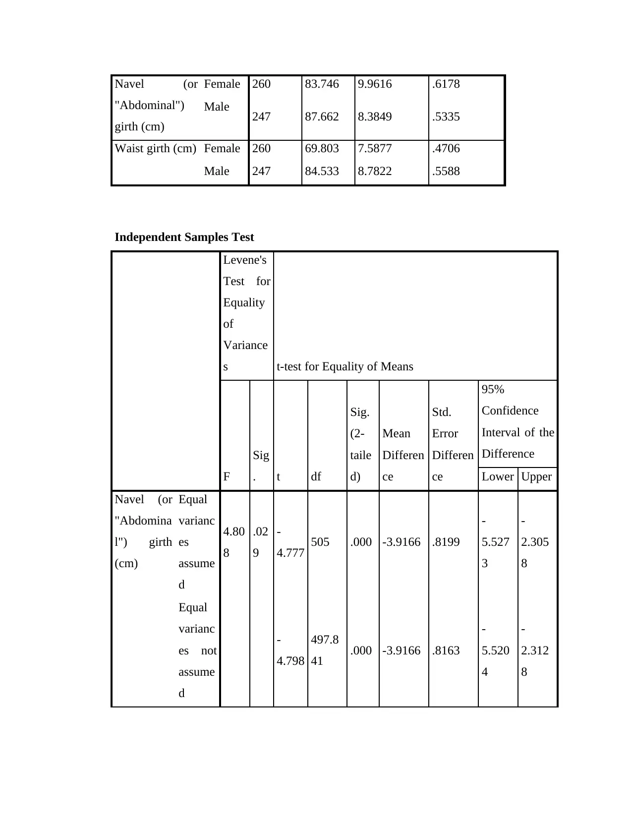
(f) Hypothesis test using T test
Group Statistics
Gender N Mean
Std.
Deviation
Std. Error
Mean
⊘ This is a preview!⊘
Do you want full access?
Subscribe today to unlock all pages.

Trusted by 1+ million students worldwide
Navel (or
"Abdominal")
girth (cm)
Female 260 83.746 9.9616 .6178
Male 247 87.662 8.3849 .5335
Waist girth (cm) Female 260 69.803 7.5877 .4706
Male 247 84.533 8.7822 .5588
Independent Samples Test
Levene's
Test for
Equality
of
Variance
s t-test for Equality of Means
F
Sig
. t df
Sig.
(2-
taile
d)
Mean
Differen
ce
Std.
Error
Differen
ce
95%
Confidence
Interval of the
Difference
Lower Upper
Navel (or
"Abdomina
l") girth
(cm)
Equal
varianc
es
assume
d
4.80
8
.02
9
-
4.777 505 .000 -3.9166 .8199
-
5.527
3
-
2.305
8
Equal
varianc
es not
assume
d
-
4.798
497.8
41 .000 -3.9166 .8163
-
5.520
4
-
2.312
8
Paraphrase This Document
Need a fresh take? Get an instant paraphrase of this document with our AI Paraphraser
Waist girth
(cm)
Equal
varianc
es
assume
d
8.04
4
.00
5
-
20.23
8
505 .000 -
14.7297 .7278
-
16.15
97
-
13.29
98
Equal
varianc
es not
assume
d
-
20.16
3
486.3
21 .000 -
14.7297 .7305
-
16.16
52
-
13.29
43
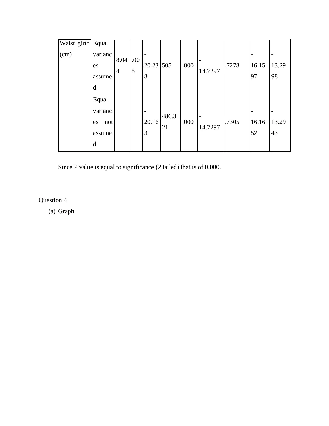
Since P value is equal to significance (2 tailed) that is of 0.000.
Question 4
(a) Graph
(cm)
Equal
varianc
es
assume
d
8.04
4
.00
5
-
20.23
8
505 .000 -
14.7297 .7278
-
16.15
97
-
13.29
98
Equal
varianc
es not
assume
d
-
20.16
3
486.3
21 .000 -
14.7297 .7305
-
16.16
52
-
13.29
43
Since P value is equal to significance (2 tailed) that is of 0.000.
Question 4
(a) Graph

(b) Analysis- The above chart indicates about knee girth over patella of male and female.
The knee girth information is given in centimeter. The graph indicates that there are more
numbers of male as compared to female. In addition to this, higher knee girth is above
41.5 cm while the lowest girth is of 29.0 cm.
(c) ∑= female participants (Knee girth over patella)<male participants (Knee girth over
patella)
(d) Assumption: “Body structure of male is stronger than female thus knee girth of male is
wider than female’s knee girth”
(e) Calculation without SPSS:
Mean: Total of male and female knee girth / number of male and female
= 36.20
Mode: Value which has higher frequency
⊘ This is a preview!⊘
Do you want full access?
Subscribe today to unlock all pages.

Trusted by 1+ million students worldwide
= 35.6
Standard deviation:
= 2.62
(f) The P value is 6.845 (approx). This value is calculated in accordance of regression model
in which multiple R= 0.37, R2= 0.14, SS= 474.54 and significant f= 6.85e-18.
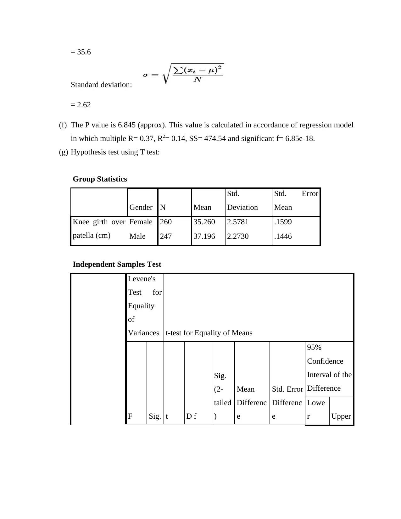
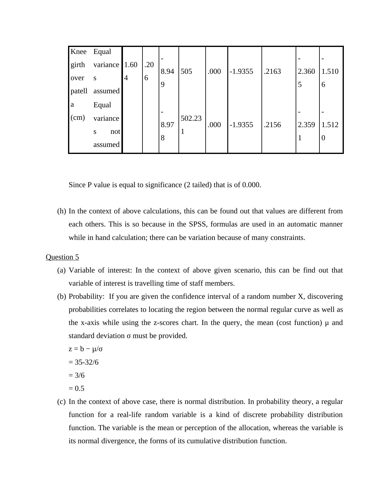
(g) Hypothesis test using T test:
Group Statistics
Gender N Mean
Std.
Deviation
Std. Error
Mean
Knee girth over
patella (cm)
Female 260 35.260 2.5781 .1599
Male 247 37.196 2.2730 .1446
Independent Samples Test
Levene's
Test for
Equality
of
Variances t-test for Equality of Means
F Sig. t D f
Sig.
(2-
tailed
)
Mean
Differenc
e
Std. Error
Differenc
e
95%
Confidence
Interval of the
Difference
Lowe
r Upper
Paraphrase This Document
Need a fresh take? Get an instant paraphrase of this document with our AI Paraphraser
Knee
girth
over
patell
a
(cm)
Equal
variance
s
assumed
1.60
4
.20
6
-
8.94
9
505 .000 -1.9355 .2163
-
2.360
5
-
1.510
6
Equal
variance
s not
assumed
-
8.97
8
502.23
1 .000 -1.9355 .2156
-
2.359
1
-
1.512
0
Since P value is equal to significance (2 tailed) that is of 0.000.
(h) In the context of above calculations, this can be found out that values are different from
each others. This is so because in the SPSS, formulas are used in an automatic manner
while in hand calculation; there can be variation because of many constraints.
Question 5
(a) Variable of interest: In the context of above given scenario, this can be find out that
variable of interest is travelling time of staff members.
(b) Probability: If you are given the confidence interval of a random number X, discovering
probabilities correlates to locating the region between the normal regular curve as well as
the x-axis while using the z-scores chart. In the query, the mean (cost function) μ and
standard deviation σ must be provided.
z = b − μ/σ
= 35-32/6
= 3/6
= 0.5
(c) In the context of above case, there is normal distribution. In probability theory, a regular
function for a real-life random variable is a kind of discrete probability distribution
function. The variable is the mean or perception of the allocation, whereas the variable is
its normal divergence, the forms of its cumulative distribution function.
(d) Calculation of probability if the sample mean of the random sample of daily travelling
times of 9 staff will be less than 32 minutes:
Probability: 35-32/9
= 3/9
= 0.33
(e) The reason due to which there is difference in probability in both cases is that in part b
number of staff members was selected on a random basis. While in section d, number of
staff members were certain and not selected on random base.
⊘ This is a preview!⊘
Do you want full access?
Subscribe today to unlock all pages.

Trusted by 1+ million students worldwide
1 out of 12
Your All-in-One AI-Powered Toolkit for Academic Success.
+13062052269
info@desklib.com
Available 24*7 on WhatsApp / Email
![[object Object]](/_next/static/media/star-bottom.7253800d.svg)
Unlock your academic potential
Copyright © 2020–2026 A2Z Services. All Rights Reserved. Developed and managed by ZUCOL.