Statistics Question Solution 2022

Hello dears, Hope this massage finds you well and safe, need an expert fill these question attached with a professional and managerial statistics answers Thanks

STATISTICS
STUDENT ID:
[Pick the date]

Question 1
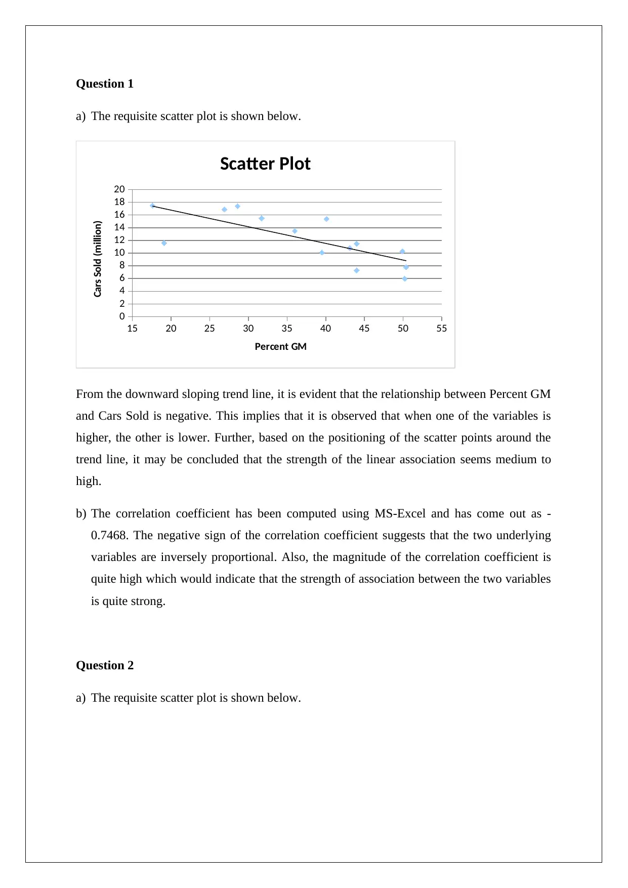
a) The requisite scatter plot is shown below.
15 20 25 30 35 40 45 50 55
0
2
4
6
8
10
12
14
16
18
20
Scatter Plot
Percent GM
Cars Sold (million)
From the downward sloping trend line, it is evident that the relationship between Percent GM
and Cars Sold is negative. This implies that it is observed that when one of the variables is
higher, the other is lower. Further, based on the positioning of the scatter points around the
trend line, it may be concluded that the strength of the linear association seems medium to
high.
b) The correlation coefficient has been computed using MS-Excel and has come out as -
0.7468. The negative sign of the correlation coefficient suggests that the two underlying
variables are inversely proportional. Also, the magnitude of the correlation coefficient is
quite high which would indicate that the strength of association between the two variables
is quite strong.
Question 2
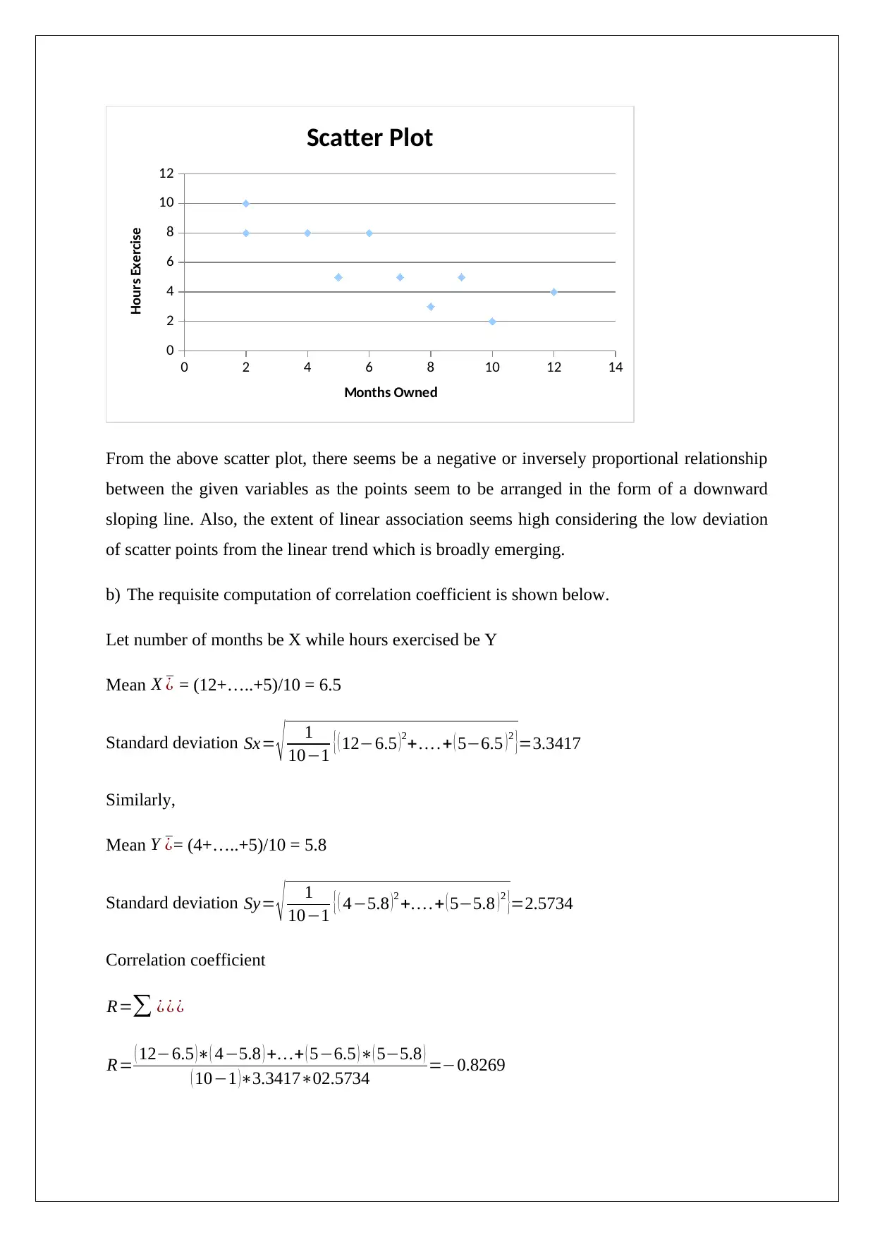
a) The requisite scatter plot is shown below.

0 2 4 6 8 10 12 14
0
2
4
6
8
10
12
Scatter Plot
Months Owned
Hours Exercise
From the above scatter plot, there seems be a negative or inversely proportional relationship
between the given variables as the points seem to be arranged in the form of a downward
sloping line. Also, the extent of linear association seems high considering the low deviation
of scatter points from the linear trend which is broadly emerging.
b) The requisite computation of correlation coefficient is shown below.
Let number of months be X while hours exercised be Y
Mean X ¯¿ = (12+…..+5)/10 = 6.5
Standard deviation Sx= √ 1
10−1 { ( 12−6.5 ) 2+… .+ ( 5−6.5 ) 2 }=3.3417
Similarly,
Mean Y ¯¿= (4+…..+5)/10 = 5.8
Standard deviation Sy= √ 1
10−1 { ( 4−5.8 )2 +… .+ ( 5−5.8 )2 }=2.5734
Correlation coefficient
R=∑ ¿ ¿ ¿
R= ( 12−6.5 )∗( 4−5.8 ) +…+ ( 5−6.5 )∗( 5−5.8 )
( 10−1 )∗3.3417∗02.5734 =−0.8269

From the above computation, it is evident that there is a very strong negative correlation
between the given variables.
Question 3
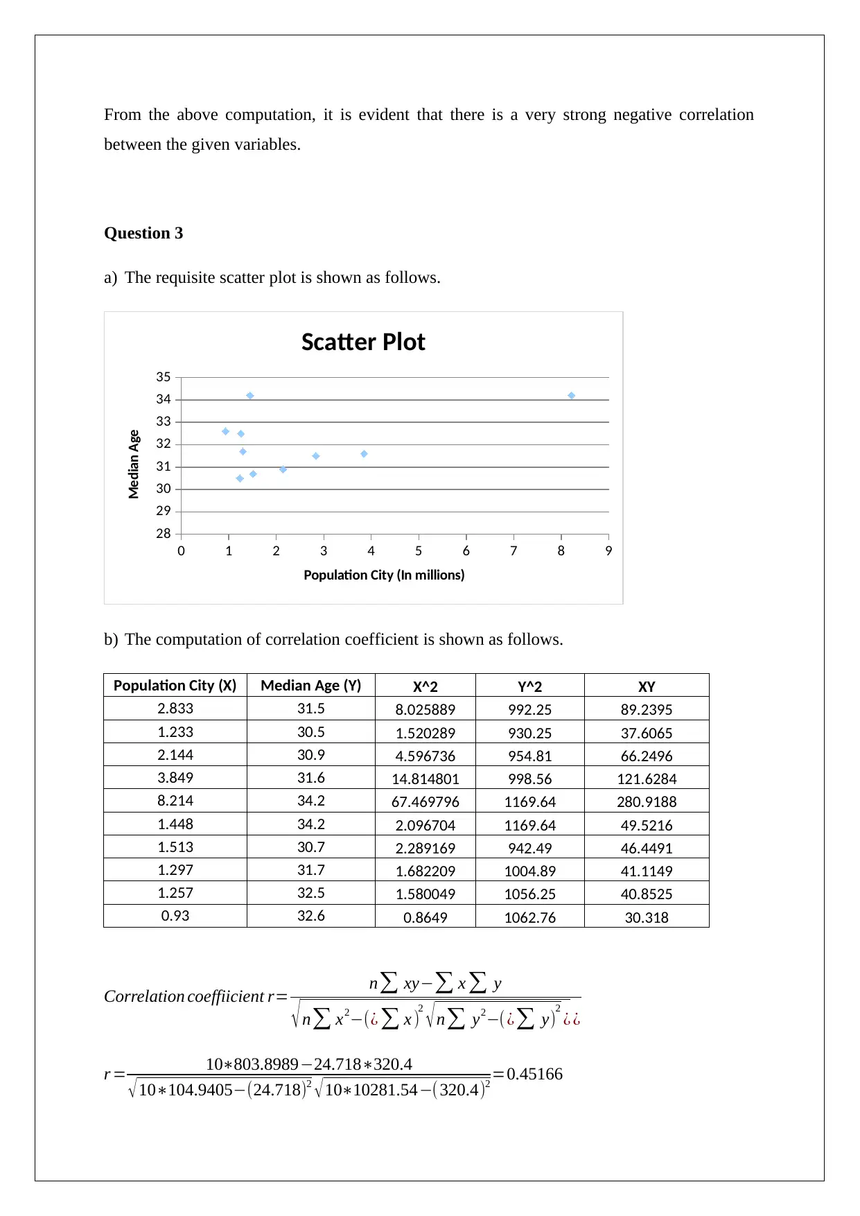
a) The requisite scatter plot is shown as follows.
0 1 2 3 4 5 6 7 8 9
28
29
30
31
32
33
34
35
Scatter Plot
Population City (In millions)
Median Age
b) The computation of correlation coefficient is shown as follows.
Population City (X) Median Age (Y) X^2 Y^2 XY
2.833 31.5 8.025889 992.25 89.2395
1.233 30.5 1.520289 930.25 37.6065
2.144 30.9 4.596736 954.81 66.2496
3.849 31.6 14.814801 998.56 121.6284
8.214 34.2 67.469796 1169.64 280.9188
1.448 34.2 2.096704 1169.64 49.5216
1.513 30.7 2.289169 942.49 46.4491
1.297 31.7 1.682209 1004.89 41.1149
1.257 32.5 1.580049 1056.25 40.8525
0.93 32.6 0.8649 1062.76 30.318
Correlation coeffiicient r= n∑ xy−∑ x ∑ y
√ n∑ x2−(¿ ∑ x )2
√ n∑ y2−( ¿∑ y)2
¿ ¿
r = 10∗803.8989−24.718∗320.4
√ 10∗104.9405−(24.718)2
√ 10∗10281.54−( 320.4)2 =0.45166

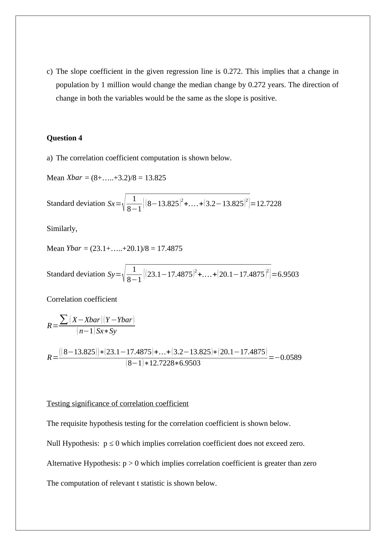
c) The slope coefficient in the given regression line is 0.272. This implies that a change in
population by 1 million would change the median change by 0.272 years. The direction of
change in both the variables would be the same as the slope is positive.
Question 4
a) The correlation coefficient computation is shown below.
Mean Xbar = (8+…..+3.2)/8 = 13.825
Standard deviation Sx= √ 1
8−1 { ( 8−13.825 ) 2 +… .+ ( 3.2−13.825 ) 2 }=12.7228
Similarly,
Mean Ybar = (23.1+…..+20.1)/8 = 17.4875
Standard deviation Sy= √ 1
8−1 { ( 23.1−17.4875 )2 +… .+ ( 20.1−17.4875 )2 }=6.9503
Correlation coefficient
R=∑ ( X−Xbar ) ( Y −Ybar )
( n−1 ) Sx∗Sy
R= ( ( 8−13.825 ) )∗( 23.1−17.4875 ) +…+ ( 3.2−13.825 )∗ ( 20.1−17.4875 )
( 8−1 )∗12.7228∗6.9503 =−0.0589
Testing significance of correlation coefficient
The requisite hypothesis testing for the correlation coefficient is shown below.
Null Hypothesis: p ≤ 0 which implies correlation coefficient does not exceed zero.
Alternative Hypothesis: p > 0 which implies correlation coefficient is greater than zero
The computation of relevant t statistic is shown below.

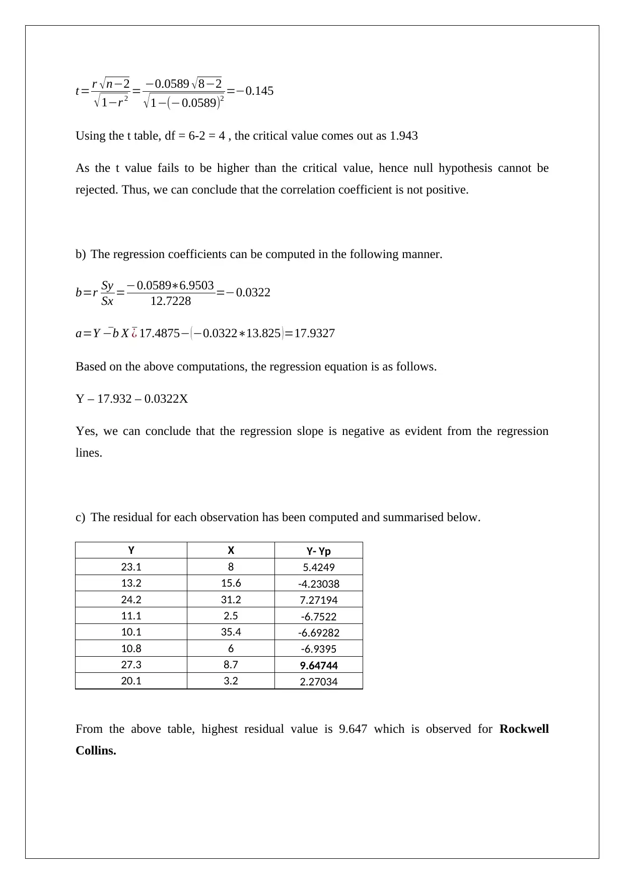
t= r √n−2
√1−r 2 = −0.0589 √8−2
√1−(−0.0589)2 =−0.145
Using the t table, df = 6-2 = 4 , the critical value comes out as 1.943
As the t value fails to be higher than the critical value, hence null hypothesis cannot be
rejected. Thus, we can conclude that the correlation coefficient is not positive.
b) The regression coefficients can be computed in the following manner.
b=r Sy
Sx =−0.0589∗6.9503
12.7228 =−0.0322
a=Y ¯−b X ¯¿ 17.4875− (−0.0322∗13.825 )=17.9327
Based on the above computations, the regression equation is as follows.
Y – 17.932 – 0.0322X
Yes, we can conclude that the regression slope is negative as evident from the regression
lines.
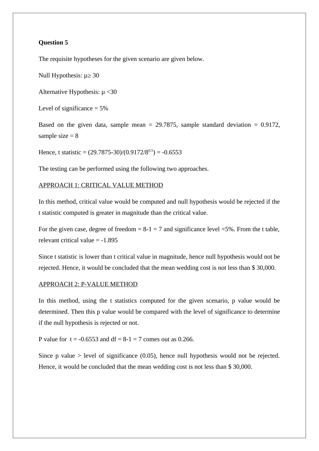
c) The residual for each observation has been computed and summarised below.
Y X Y- Yp
23.1 8 5.4249
13.2 15.6 -4.23038
24.2 31.2 7.27194
11.1 2.5 -6.7522
10.1 35.4 -6.69282
10.8 6 -6.9395
27.3 8.7 9.64744
20.1 3.2 2.27034
From the above table, highest residual value is 9.647 which is observed for Rockwell
Collins.

Question 5
The requisite hypotheses for the given scenario are given below.
Null Hypothesis: μ≥ 30
Alternative Hypothesis: μ <30
Level of significance = 5%
Based on the given data, sample mean = 29.7875, sample standard deviation = 0.9172,
sample size = 8
Hence, t statistic = (29.7875-30)/(0.9172/80.5) = -0.6553
The testing can be performed using the following two approaches.
APPROACH 1: CRITICAL VALUE METHOD
In this method, critical value would be computed and null hypothesis would be rejected if the
t statistic computed is greater in magnitude than the critical value.
For the given case, degree of freedom = 8-1 = 7 and significance level =5%. From the t table,
relevant critical value = -1.895
Since t statistic is lower than t critical value in magnitude, hence null hypothesis would not be
rejected. Hence, it would be concluded that the mean wedding cost is not less than $ 30,000.
APPROACH 2: P-VALUE METHOD
In this method, using the t statistics computed for the given scenario, p value would be
determined. Then this p value would be compared with the level of significance to determine
if the null hypothesis is rejected or not.
P value for t = -0.6553 and df = 8-1 = 7 comes out as 0.266.
Since p value > level of significance (0.05), hence null hypothesis would not be rejected.
Hence, it would be concluded that the mean wedding cost is not less than $ 30,000.