Ecological Conditions of Barker's Creek Circuit: A Scientific Report
VerifiedAdded on 2022/09/27
|27
|4773
|19
Report
AI Summary
This scientific report presents an investigation into the ecological conditions of Barker's Creek Circuit in Bunya Mountains National Park, focusing on the differences between various habitat types. The study, conducted as part of the BVB204 course, examines abiotic factors, transect data, and quadrat data across six zones, including microphyll rainforest, mesophyll rainforest, notophyll rainforest, grassland bald, and sclerophyll eucalypt woodland. The report utilizes ANOVA and linear regression to analyze data, specifically investigating differences in soil pH, leaf litter cover, tree height, and the relationship between canopy layers and humidity. Results from R studio are presented, including summary statistics, ANOVA tests, and linear regression models. The report includes figures, tables, and a discussion interpreting the findings in the context of scientific literature, addressing specific research questions and providing a comprehensive analysis of the ecosystem's characteristics.

Running Head: ECOLOGICAL CONDITIONS OF BARKER’S CREEK CIRCUIT
1
AN INVESTIGATION OF ECOLOGICAL CONDITIONS OF BARKER’S CREEK CIRCUIT
Name of the institution:
Name of student:
Date:
1
AN INVESTIGATION OF ECOLOGICAL CONDITIONS OF BARKER’S CREEK CIRCUIT
Name of the institution:
Name of student:
Date:
Paraphrase This Document
Need a fresh take? Get an instant paraphrase of this document with our AI Paraphraser

ECOLOGICAL CONDITIONS OF BARKER’S CREEK CIRCUIT
2
Table of Contents
Introduction.................................................................................................................................................3
Literature Review....................................................................................................................................3
Methods.......................................................................................................................................................6
Study site.................................................................................................................................................6
Data collection.........................................................................................................................................6
Data-analyses...........................................................................................................................................6
Results.........................................................................................................................................................7
Results section from R studio..................................................................................................................7
Summary Statistics..............................................................................................................................7
ANOVA Test.......................................................................................................................................7
Linear Regression..............................................................................................................................11
Graphical Analysis............................................................................................................................16
Discussion.................................................................................................................................................20
References.................................................................................................................................................23
ECOLOGICAL CONDITIONS OF BARKER’S CREEK CIRCUIT
3
Introduction
Ecosystem is the mutual existence of plants and animals in the environment. The
existence of plants and animals in the setting of an ecosystem is meant to be a benefit to both the
parties. Some of the major benefits of ecosystem include: Economic benefits to human beings,
protection of the rare and endangered species, foundation of sustainable development and the
essential of the ecosystem to the survival of human being and plants (Andrew, Thomas, Kristin,
& Cristine, 2013).
Literature Review
The existence of proper forest covers in the environment has great economic benefits to
human beings. Forest provides vast majority of the raw materials that used in the manufacturing
industry. For example, paper and other stationaries like pencil are products of trees. Similarly,
plants, are a source of rain. The rain can be used to generate hydroelectricity that is consumed
both at home and in the industries. Tourism has a direct contribution to the economy since the
tourist pay for their visit to the tourism attraction sites (Youngentob, Likens, Williams, &
Lindenmayer, 2012).
Ecosystem is a foundation of sustainable development. Sustainable development is about
the proper and responsible utilization of the available resources for the good of the future.
Ecosystem ensures that there is economic sustainability by providing the necessary raw materials
that are required in the industries. Similarly, ecosystem is a foundation of sustainable
development by ensuring that there is no change in climatic conditions. Therefore, the farming
systems and practices are maintained ensuring that there is a constant supply of food and raw
materials for the manufactured goods (Shishi & Katia, 2013).
⊘ This is a preview!⊘
Do you want full access?
Subscribe today to unlock all pages.
Trusted by 1+ million students worldwide
ECOLOGICAL CONDITIONS OF BARKER’S CREEK CIRCUIT
4
Ecosystem is fundamental for the survival of human beings and plants. The mutual
existence of plants and animals ensures that the rare species do not become endangered or
extinct. It is the responsibility of human beings to protect the rare species of plants and animals
to maintain their sustainability. The endangered species of plants and animals are extremely
beneficial to human beings since they hugely attract tourists thereby leading to more income
(Perkol-Finkel, et al., 2010).
The characteristics that make up ecosystems include biodiversity, energy flow, regular
temperature, regular soil pH and regular humidity. Biodiversity is the existence of several or
numerous species of plants and animals in the same ecosystem. Biodiversity can be maintained
by ensuring that all species of plants and animals are properly protected. Biodiversity ensures
that both animals and plants co-exist without any party causing troubles to the other (Jung, et al.,
2014). The structure of an ecosystem is highly dependent on the diversity of the species in that
ecosystem. Therefore, the ecosystems with more diverse species have are highly complex while
an ecosystem with few diverse species have a less complex ecosystem (Cooper, et al., 2017).
An ecosystem has a regular temperature. The existence of regular temperature ensures
that the ecosystem is conducive enough to sustain the existing plants and animals. Therefore, the
activities that may cause alterations to the regular temperature must be avoided at all costs. The
major cause of alterations to the regular temperature is the change in climate. The change in
climate of an ecosystem can be as a result of several factors like the excessive release of carbon
dioxide into the atmosphere (Intsone & Lesley, 2014).
An ecosystem must have a regular soil pH. Soil pH is the degree of acidity or the
alkalinity of the soil. Different plants and different animals exist under different soil pH. The
Paraphrase This Document
Need a fresh take? Get an instant paraphrase of this document with our AI Paraphraser

ECOLOGICAL CONDITIONS OF BARKER’S CREEK CIRCUIT
5
underground animals must have a regular soil p in order to survive. Similarly, the plants must
have a regular soil pH in order to experience a proper growth (Inger, et al., 2014).
An ecosystem must have a regular humidity. Humidity is the amount of water vapor that
is in the atmosphere. Different plants and different animals require different levels of humidity in
order to properly thrive in the ecosystem. Therefore, an ecosystem will only exist in an
environment where there is no climate change (Cynthia, Robert, Nico, & Roderic, 2012).
The other important characteristic of an ecosystem is the energy flow. Energy flow refers
to the amount of energy that is transferred among the members of the ecosystem I. e. energy flow
from plants to animals and vice versa. The complexity and amount of energy flow in an
ecosystem depends on the complexity of the ecosystem (Andrew, Thomas, Kristin, & Cristine,
2013).
More complex ecosystems with a more diverse species of animals and plants have more
energy flow that the simple ecosystems with less diverse species of plants and animals. However,
the extent of energy fixation in an ecosystem are limited and cannot be altered without causing
serous damages to the ecosystem. Therefore, any changes in the environment that may lead to
the alteration in energy flow can affect the ecosystem in diverse ways. The effects may even lead
to the extinction of some species of plants and animals that are very dear to the ecosystem
(Andrew, Thomas, Kristin, & Cristine, 2013).
The characteristics listed above clearly demonstrate that ecosystem is a major structural
and functional unit of ecology. Therefore, ecosystem must be maintained in order to maintain a
proper ecology.
This research was conducted in Barker’s Creek Circuit, Bunya Mountains National Park,
South-East Queensland. Barker Creek Circuit is a 10.5 Kilometer loop trail. The loop is
ECOLOGICAL CONDITIONS OF BARKER’S CREEK CIRCUIT
6
moderately trafficked. The loop is located in the state of Queensland, Australia. From the
information that was collected, the research seeks to answer a number of specific questions.
Some of the specific research questions include: Is there any significant difference in the average
soil pH across the different habitat types? Is there any significant difference in the average level
of leaf litter cover across the different habitat types? Can predict the predict the number of layers
of a canopy can be predicted based on the humidity of the canopy? Is there any significant
difference in the average height of a tree across the different types of habitats?
Methods
Study site
The study site was Barker’s Creek Circuit, Bunya Mountains National Park, South-East
Queensland. Barker Creek Circuit is a 10.5 Kilometer loop trail. The loop is moderately
trafficked. The loop is located in the state of Queensland, Australia. The loop offers scenic views
and it primary used for hiking, nature trips, walking, and bird watching. The study site was
divided into six major zones from where the data was collected. The six zones were microphyll
rainforest, mesophyll rainforest, notophyll rainforest, grassland bald, and sclerophyll eucalypt
woodland.
Data collection
The three types of data that were collected are abiotic data, transect data and the quadrat
data. The abiotic data were measured in terms of the intensity of light, humidity, wind,
temperature, GPS Coordinates, elevation (m), topography and soil characteristics (pH, soil
structure and basic surface geology).
⊘ This is a preview!⊘
Do you want full access?
Subscribe today to unlock all pages.
Trusted by 1+ million students worldwide

ECOLOGICAL CONDITIONS OF BARKER’S CREEK CIRCUIT
7
Data-analyses
Analysis of variance (ANOVA) is a statistical technique that is used to investigate whether there
exists any significant difference in the average values of variables under study. Analysis of
variance test was conducted to investigate whether there is any significant difference in the
average soil pH across the different habitat types. Similarly, analysis of variance (ANOVA) was
conducted to investigate whether there was any significant difference in the average level of leaf
litter cover across the different habitat types.
Linear regression is statistical technique that is used to generate a linear model for predicting
variables. A regression analysis was conducted to determine whether the number of layers of a
canopy can be predicted based on the humidity of the canopy.
Results
Results section from R studio
Summary Statistics
The following code and output were used to display the summary statistics of number of canopy
layers, the leaf litter cover, the intensity of light, soil moisture, temperature and soil pH.
summary(dat2)
canopy.layers leaf.litter.cover light soil.moisture temperature soil.ph
Min. :0.000 Min. : 0.00 Min. : 1.00 Min. : 1.00 Min. : 0.00 Min. :0.000
1st Qu.:1.000 1st Qu.: 15.00 1st Qu.:17.25 1st Qu.:16.00 1st Qu.:26.57 1st Qu.:4.000
Median :2.000 Median : 70.00 Median :35.50 Median :37.00 Median :28.60
Median :4.500
Mean :1.766 Mean : 55.25 Mean :33.75 Mean :36.48 Mean :27.77 Mean :4.266
3rd Qu.:3.000 3rd Qu.: 90.00 3rd Qu.:48.00 3rd Qu.:55.75 3rd Qu.:30.40 3rd Qu.:5.000
Paraphrase This Document
Need a fresh take? Get an instant paraphrase of this document with our AI Paraphraser
ECOLOGICAL CONDITIONS OF BARKER’S CREEK CIRCUIT
8
Max. :5.000 Max. :100.00 Max. :60.00 Max. :80.00 Max. :33.10 Max. :9.000
NA's :25 NA's :33 NA's :74 NA's :22 NA's :54
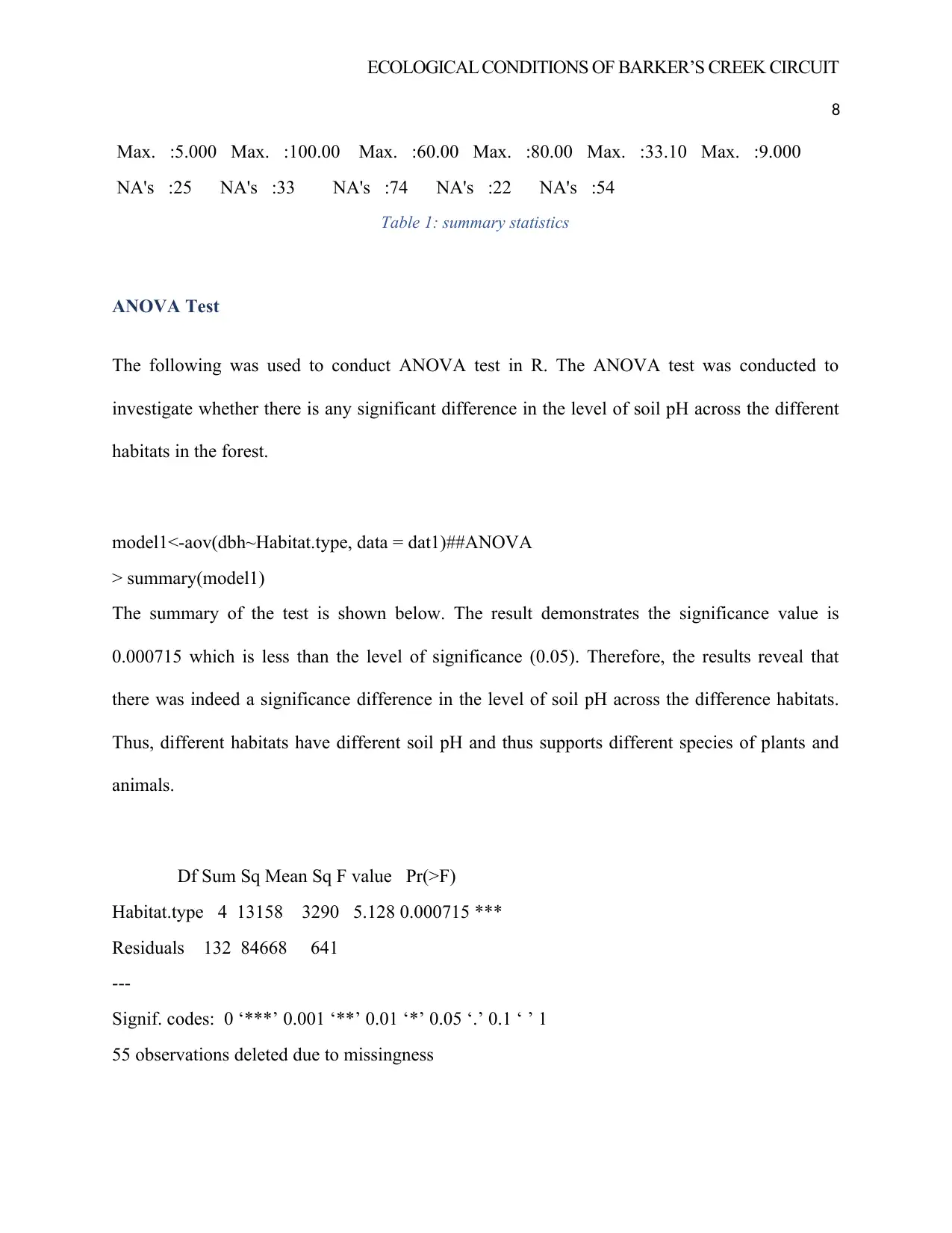
Table 1: summary statistics
ANOVA Test
The following was used to conduct ANOVA test in R. The ANOVA test was conducted to
investigate whether there is any significant difference in the level of soil pH across the different
habitats in the forest.
model1<-aov(dbh~Habitat.type, data = dat1)##ANOVA
> summary(model1)
The summary of the test is shown below. The result demonstrates the significance value is
0.000715 which is less than the level of significance (0.05). Therefore, the results reveal that
there was indeed a significance difference in the level of soil pH across the difference habitats.
Thus, different habitats have different soil pH and thus supports different species of plants and
animals.
Df Sum Sq Mean Sq F value Pr(>F)
Habitat.type 4 13158 3290 5.128 0.000715 ***
Residuals 132 84668 641
---
Signif. codes: 0 ‘***’ 0.001 ‘**’ 0.01 ‘*’ 0.05 ‘.’ 0.1 ‘ ’ 1
55 observations deleted due to missingness
8
Max. :5.000 Max. :100.00 Max. :60.00 Max. :80.00 Max. :33.10 Max. :9.000
NA's :25 NA's :33 NA's :74 NA's :22 NA's :54
Table 1: summary statistics
ANOVA Test
The following was used to conduct ANOVA test in R. The ANOVA test was conducted to
investigate whether there is any significant difference in the level of soil pH across the different
habitats in the forest.
model1<-aov(dbh~Habitat.type, data = dat1)##ANOVA
> summary(model1)
The summary of the test is shown below. The result demonstrates the significance value is
0.000715 which is less than the level of significance (0.05). Therefore, the results reveal that
there was indeed a significance difference in the level of soil pH across the difference habitats.
Thus, different habitats have different soil pH and thus supports different species of plants and
animals.
Df Sum Sq Mean Sq F value Pr(>F)
Habitat.type 4 13158 3290 5.128 0.000715 ***
Residuals 132 84668 641
---
Signif. codes: 0 ‘***’ 0.001 ‘**’ 0.01 ‘*’ 0.05 ‘.’ 0.1 ‘ ’ 1
55 observations deleted due to missingness

ECOLOGICAL CONDITIONS OF BARKER’S CREEK CIRCUIT
9
The following R code was used to investigate whether there was any significant difference in the
average level of leaf litter cover across the different habitat types.
model9<-aov(leaf.litter.cover~Habitat.type, data = dat1)
> summary(model9)
The following are the analysis result of the ANOVA test. From the results, the p- value is <2e-16
which is less than the level of significance (0.05). Therefore, it is clear that there a significant
difference in the level of leaf litter cover across the difference habitat types.
Df Sum Sq Mean Sq F value Pr(>F)
Habitat.type 4 131836 32959 46.3 <2e-16 ***
Residuals 154 109616 712
---
Signif. codes: 0 ‘***’ 0.001 ‘**’ 0.01 ‘*’ 0.05 ‘.’ 0.1 ‘ ’ 1
33 observations deleted due to missingness
model4<-aov(tree.height~Habitat.type, data = dat1)
> summary(model4)
Df Sum Sq Mean Sq F value Pr(>F)
Habitat.type 4 757.3 189.33 6.539 9.64e-05 ***
Residuals 106 3069.4 28.96
---
Signif. codes: 0 ‘***’ 0.001 ‘**’ 0.01 ‘*’ 0.05 ‘.’ 0.1 ‘ ’ 1
81 observations deleted due to missingness
> TukeyHSD(model4)
⊘ This is a preview!⊘
Do you want full access?
Subscribe today to unlock all pages.
Trusted by 1+ million students worldwide

ECOLOGICAL CONDITIONS OF BARKER’S CREEK CIRCUIT
10
Tukey multiple comparisons of means
95% family-wise confidence level
The following code was used to investigate whether there exists any significant difference in the
average height of a tree and the type of habitat. The results demonstrate that the p- values are all
less than the level of significance (0.05). Therefore, it is clear that there exists a significant
difference in the average height of a tree across the difference types of habitat.
Fit: aov(formula = tree.height ~ Habitat.type, data = dat1)
$Habitat.type
diff lwr upr p adj
Rainforest-Heathland 5.084152 1.3168249 8.8514782 0.0026656
Sand dune-Heathland -2.698682 -7.7329838 2.3356202 0.5726955
Sand dune Scrub-Heathland -2.698682 -9.8655667 4.4682030 0.8337468
Woodland-Heathland 1.436557 -2.2988058 5.1719195 0.8227986
Sand dune-Rainforest -7.782833 -12.8838177 -2.6818489 0.0004628
Sand dune Scrub-Rainforest -7.782833 -14.9967147 -0.5689520 0.0277027
Woodland-Rainforest -3.647595 -7.4723534 0.1771641 0.0692266
Sand dune Scrub-Sand dune 0.000000 -7.9493101 7.9493101 1.0000000
Woodland-Sand dune 4.135239 -0.9421844 9.2126619 0.1661766
Woodland-Sand dune Scrub 4.135239 -3.0620016 11.3324790 0.5041767
Table 2: summary ANOVA
modelhabitat<-(aov(soil.ph~Habitat.type, data=dat1))
> summary(modelhabitat)
Df Sum Sq Mean Sq F value Pr(>F)
Habitat.type 4 71.0 17.739 7.657 9.82e-06 ***
Paraphrase This Document
Need a fresh take? Get an instant paraphrase of this document with our AI Paraphraser
ECOLOGICAL CONDITIONS OF BARKER’S CREEK CIRCUIT
11
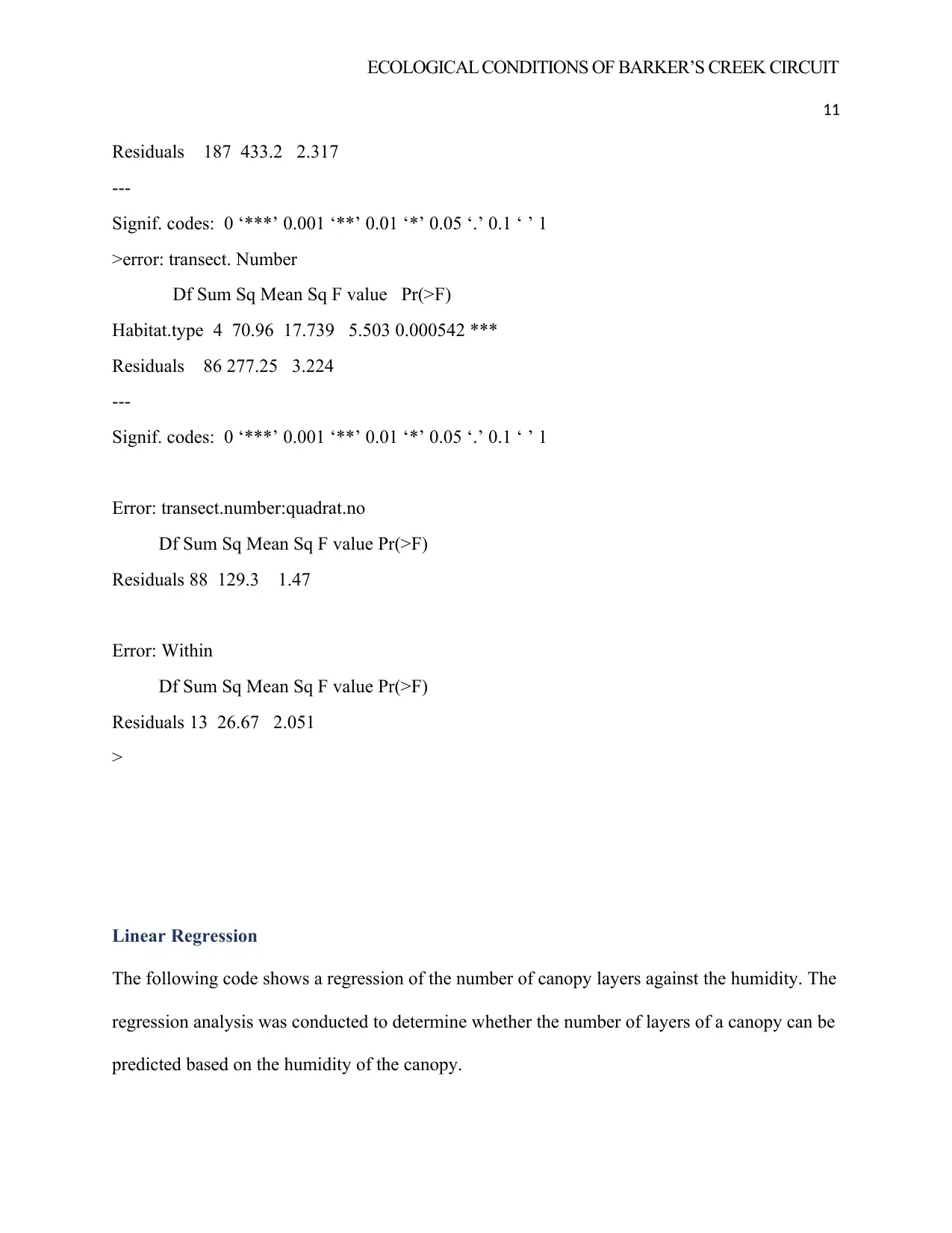
Residuals 187 433.2 2.317
---
Signif. codes: 0 ‘***’ 0.001 ‘**’ 0.01 ‘*’ 0.05 ‘.’ 0.1 ‘ ’ 1
>error: transect. Number
Df Sum Sq Mean Sq F value Pr(>F)
Habitat.type 4 70.96 17.739 5.503 0.000542 ***
Residuals 86 277.25 3.224
---
Signif. codes: 0 ‘***’ 0.001 ‘**’ 0.01 ‘*’ 0.05 ‘.’ 0.1 ‘ ’ 1
Error: transect.number:quadrat.no
Df Sum Sq Mean Sq F value Pr(>F)
Residuals 88 129.3 1.47
Error: Within
Df Sum Sq Mean Sq F value Pr(>F)
Residuals 13 26.67 2.051
>
Linear Regression
The following code shows a regression of the number of canopy layers against the humidity. The
regression analysis was conducted to determine whether the number of layers of a canopy can be
predicted based on the humidity of the canopy.
11
Residuals 187 433.2 2.317
---
Signif. codes: 0 ‘***’ 0.001 ‘**’ 0.01 ‘*’ 0.05 ‘.’ 0.1 ‘ ’ 1
>error: transect. Number
Df Sum Sq Mean Sq F value Pr(>F)
Habitat.type 4 70.96 17.739 5.503 0.000542 ***
Residuals 86 277.25 3.224
---
Signif. codes: 0 ‘***’ 0.001 ‘**’ 0.01 ‘*’ 0.05 ‘.’ 0.1 ‘ ’ 1
Error: transect.number:quadrat.no
Df Sum Sq Mean Sq F value Pr(>F)
Residuals 88 129.3 1.47
Error: Within
Df Sum Sq Mean Sq F value Pr(>F)
Residuals 13 26.67 2.051
>
Linear Regression
The following code shows a regression of the number of canopy layers against the humidity. The
regression analysis was conducted to determine whether the number of layers of a canopy can be
predicted based on the humidity of the canopy.
ECOLOGICAL CONDITIONS OF BARKER’S CREEK CIRCUIT
12
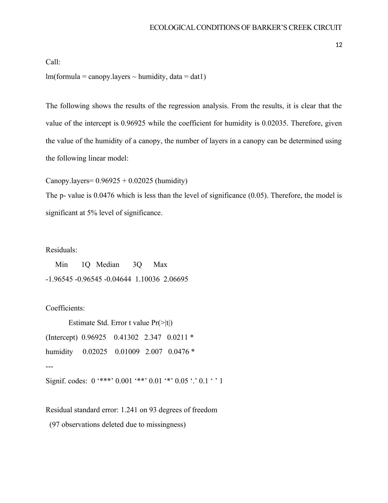
Call:
lm(formula = canopy.layers ~ humidity, data = dat1)
The following shows the results of the regression analysis. From the results, it is clear that the
value of the intercept is 0.96925 while the coefficient for humidity is 0.02035. Therefore, given
the value of the humidity of a canopy, the number of layers in a canopy can be determined using
the following linear model:
Canopy.layers= 0.96925 + 0.02025 (humidity)
The p- value is 0.0476 which is less than the level of significance (0.05). Therefore, the model is
significant at 5% level of significance.
Residuals:
Min 1Q Median 3Q Max
-1.96545 -0.96545 -0.04644 1.10036 2.06695
Coefficients:
Estimate Std. Error t value Pr(>|t|)
(Intercept) 0.96925 0.41302 2.347 0.0211 *
humidity 0.02025 0.01009 2.007 0.0476 *
---
Signif. codes: 0 ‘***’ 0.001 ‘**’ 0.01 ‘*’ 0.05 ‘.’ 0.1 ‘ ’ 1
Residual standard error: 1.241 on 93 degrees of freedom
(97 observations deleted due to missingness)
12
Call:
lm(formula = canopy.layers ~ humidity, data = dat1)
The following shows the results of the regression analysis. From the results, it is clear that the
value of the intercept is 0.96925 while the coefficient for humidity is 0.02035. Therefore, given
the value of the humidity of a canopy, the number of layers in a canopy can be determined using
the following linear model:
Canopy.layers= 0.96925 + 0.02025 (humidity)
The p- value is 0.0476 which is less than the level of significance (0.05). Therefore, the model is
significant at 5% level of significance.
Residuals:
Min 1Q Median 3Q Max
-1.96545 -0.96545 -0.04644 1.10036 2.06695
Coefficients:
Estimate Std. Error t value Pr(>|t|)
(Intercept) 0.96925 0.41302 2.347 0.0211 *
humidity 0.02025 0.01009 2.007 0.0476 *
---
Signif. codes: 0 ‘***’ 0.001 ‘**’ 0.01 ‘*’ 0.05 ‘.’ 0.1 ‘ ’ 1
Residual standard error: 1.241 on 93 degrees of freedom
(97 observations deleted due to missingness)
⊘ This is a preview!⊘
Do you want full access?
Subscribe today to unlock all pages.
Trusted by 1+ million students worldwide
1 out of 27
Related Documents


Your All-in-One AI-Powered Toolkit for Academic Success.
+13062052269
info@desklib.com
Available 24*7 on WhatsApp / Email
![[object Object]](/_next/static/media/star-bottom.7253800d.svg)
Unlock your academic potential
Copyright © 2020–2026 A2Z Services. All Rights Reserved. Developed and managed by ZUCOL.