Inference and Statistical Analysis

The assignment content consists of three statistical problems: a test for means, a test for proportions, and a test for means. In Problem 7, it is tested whether the fraction of persons who rented condominiums moved to Toronto area is greater than 0.2. The sample proportion is found to be 0.28, which is greater than 0.2, leading to rejection of the null hypothesis. In Problem 9, it is tested whether there is a significant difference in student grades under quarter and semester systems. The computed t-value is less than 1.796, leading to failure to reject the null hypothesis that the mean difference is zero. In Problem 10, it is tested whether the average value of houses sold in Victoria during the year 2001 was different from $210,200. The p-value is very small, indicating rejection of the null hypothesis.

Assignment 3
Question 1
Let
1 and
2 be the population means of useful life times (in months) of Cooper paint and King paint,
respectively. Then, the null and alternative hypotheses are:
H0 :
1 =
2
H1 :
1 ≠
2
This is a two-tailed test.
We have chosen  = 0.01.
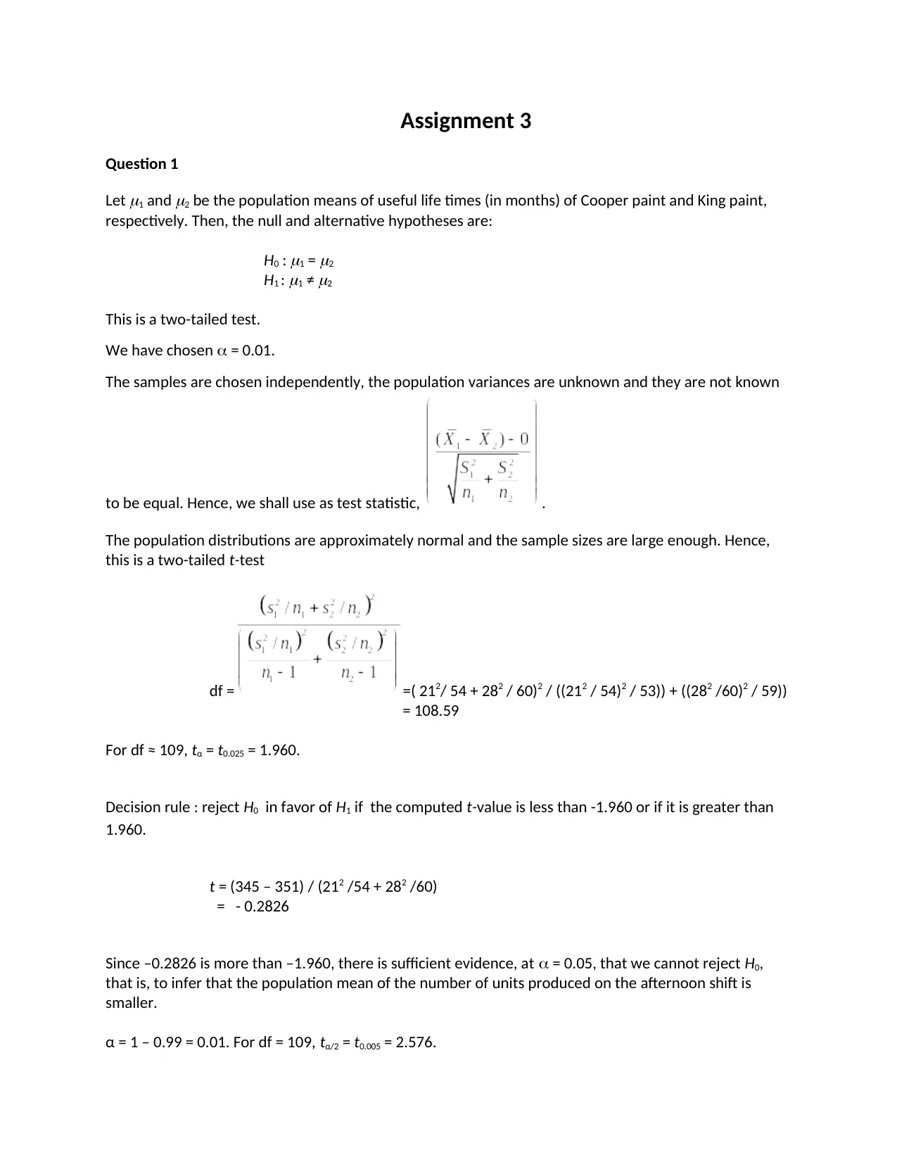
The samples are chosen independently, the population variances are unknown and they are not known
to be equal. Hence, we shall use as test statistic, .
The population distributions are approximately normal and the sample sizes are large enough. Hence,
this is a two-tailed t-test
df = =( 212/ 54 + 282 / 60)2 / ((212 / 54)2 / 53)) + ((282 /60)2 / 59))
= 108.59
For df ≈ 109, tα = t0.025 = 1.960.
Decision rule : reject H0 in favor of H1 if the computed t-value is less than -1.960 or if it is greater than
1.960.
t = (345 – 351) / (212 /54 + 282 /60)
= - 0.2826
Since –0.2826 is more than –1.960, there is sufficient evidence, at  = 0.05, that we cannot reject H0,
that is, to infer that the population mean of the number of units produced on the afternoon shift is
smaller.
α = 1 – 0.99 = 0.01. For df = 109, tα/2 = t0.005 = 2.576.

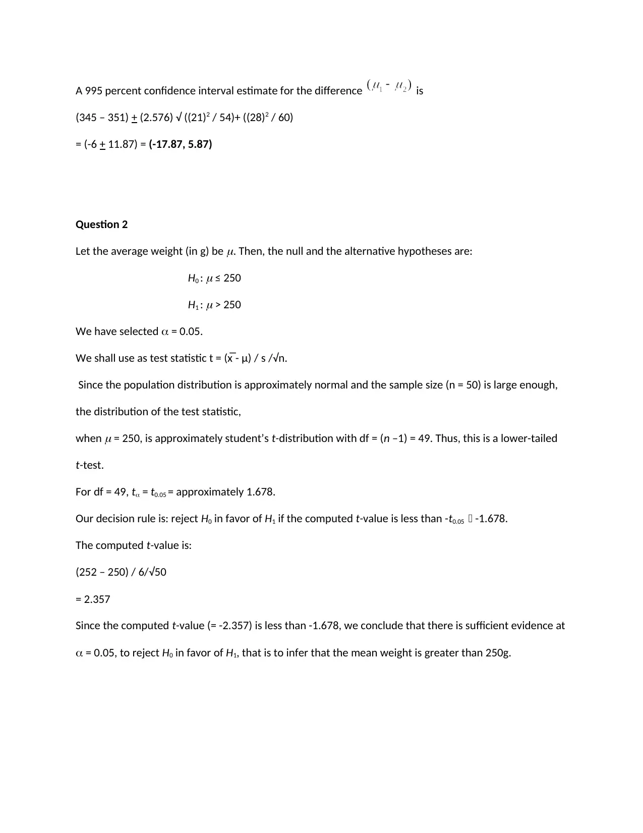
A 995 percent confidence interval estimate for the difference is
(345 – 351) + (2.576) √ ((21)2 / 54)+ ((28)2 / 60)
= (-6 + 11.87) = (-17.87, 5.87)
Question 2
Let the average weight (in g) be
. Then, the null and the alternative hypotheses are:
H0 :
 ≤ 250
H1 :
 > 250
We have selected  = 0.05.
We shall use as test statistic t = (x̅ - μ) / s /√n.
Since the population distribution is approximately normal and the sample size (n = 50) is large enough,
the distribution of the test statistic,
when
 = 250, is approximately student’s t-distribution with df = (n –1) = 49. Thus, this is a lower-tailed
t-test.
For df = 49, t = t0.05 = approximately 1.678.
Our decision rule is: reject H0 in favor of H1 if the computed t-value is less than -t0.05  -1.678.
The computed t-value is:
(252 – 250) / 6/√50
= 2.357
Since the computed t-value (= -2.357) is less than -1.678, we conclude that there is sufficient evidence at
 = 0.05, to reject H0 in favor of H1, that is to infer that the mean weight is greater than 250g.

Question 3
Let us formulate the null and alternative hypotheses.
H0: μ = $50000 (The mean income does not defer)
H1: μ ≠ $50000 (The mean income defers)
At the centre of the hypothesized distribution will be the highest possible value for which H0 could be
true, μ0 = $50000.
The significance level as given will be α = 0.1
The population standard deviation (σ) is known and the sample size is large, so the normal distribution is
appropriate and the test statistics (ᴢ) is calculated as:
z = (x̅ - μ0)/σ
= (50500 – 50000)/ (3000/√120)
= 1.825
For a two-tail z-test in which α = 0.1, z = -2.326 and z = +2.326 will be the respective boundaries for
lower and upper tails of 0.01 each. These are the critical values for the test and they identify the non
rejection and rejection regions i.e. reject H0 if calculated z < -2.326 or z > +2.326, otherwise do not
reject.
The calculated value, z = 1.825 falls within the non rejection region of the diagram. So at the 0.1 level of
significance, the null hypothesis is not rejected.
The results suggest that the mean income defers from $50000
P-value = (-1.825≤Z ≤ 1.825) = approximately 2*(1 – 0.96562) = 0.06876.

Question 4
a) True.
b) True.
c) False.
d) True.
e) True.

Question 5
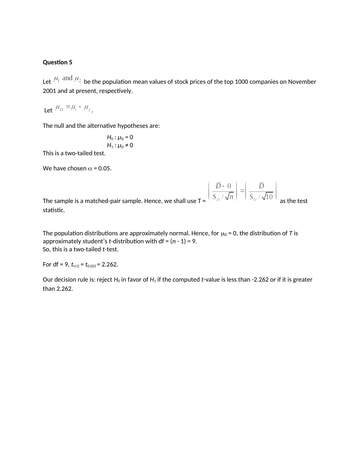
Let be the population mean values of stock prices of the top 1000 companies on November
2001 and at present, respectively.
Let .
The null and the alternative hypotheses are:
H0 : μD = 0
H1 : μD ≠ 0
This is a two-tailed test.
We have chosen  = 0.05.
The sample is a matched-pair sample. Hence, we shall use T = as the test
statistic.
The population distributions are approximately normal. Hence, for D = 0, the distribution of T is
approximately student’s t-distribution with df = (n - 1) = 9.
So, this is a two-tailed t-test.
For df = 9, t/2 = t0.025 = 2.262.
Our decision rule is: reject H0 in favor of H1 if the computed t-value is less than -2.262 or if it is greater
than 2.262.

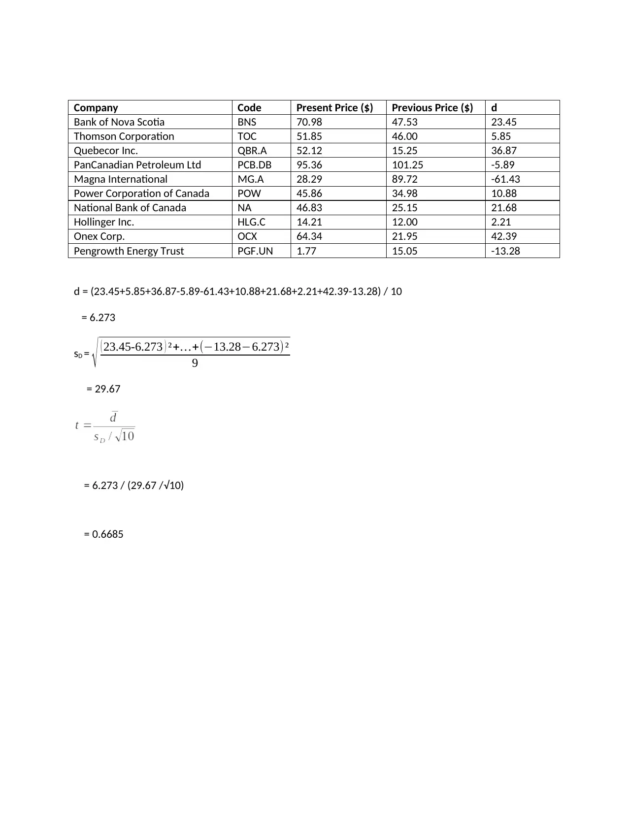
Company Code Present Price ($) Previous Price ($) d
Bank of Nova Scotia BNS 70.98 47.53 23.45
Thomson Corporation TOC 51.85 46.00 5.85
Quebecor Inc. QBR.A 52.12 15.25 36.87
PanCanadian Petroleum Ltd PCB.DB 95.36 101.25 -5.89
Magna International MG.A 28.29 89.72 -61.43
Power Corporation of Canada POW 45.86 34.98 10.88
National Bank of Canada NA 46.83 25.15 21.68
Hollinger Inc. HLG.C 14.21 12.00 2.21
Onex Corp. OCX 64.34 21.95 42.39
Pengrowth Energy Trust PGF.UN 1.77 15.05 -13.28
d = (23.45+5.85+36.87-5.89-61.43+10.88+21.68+2.21+42.39-13.28) / 10
= 6.273
sD = √ ( 23.45-6.273 ) ²+…+(−13.28−6.273) ²
9
= 29.67
= 6.273 / (29.67 /√10)
= 0.6685

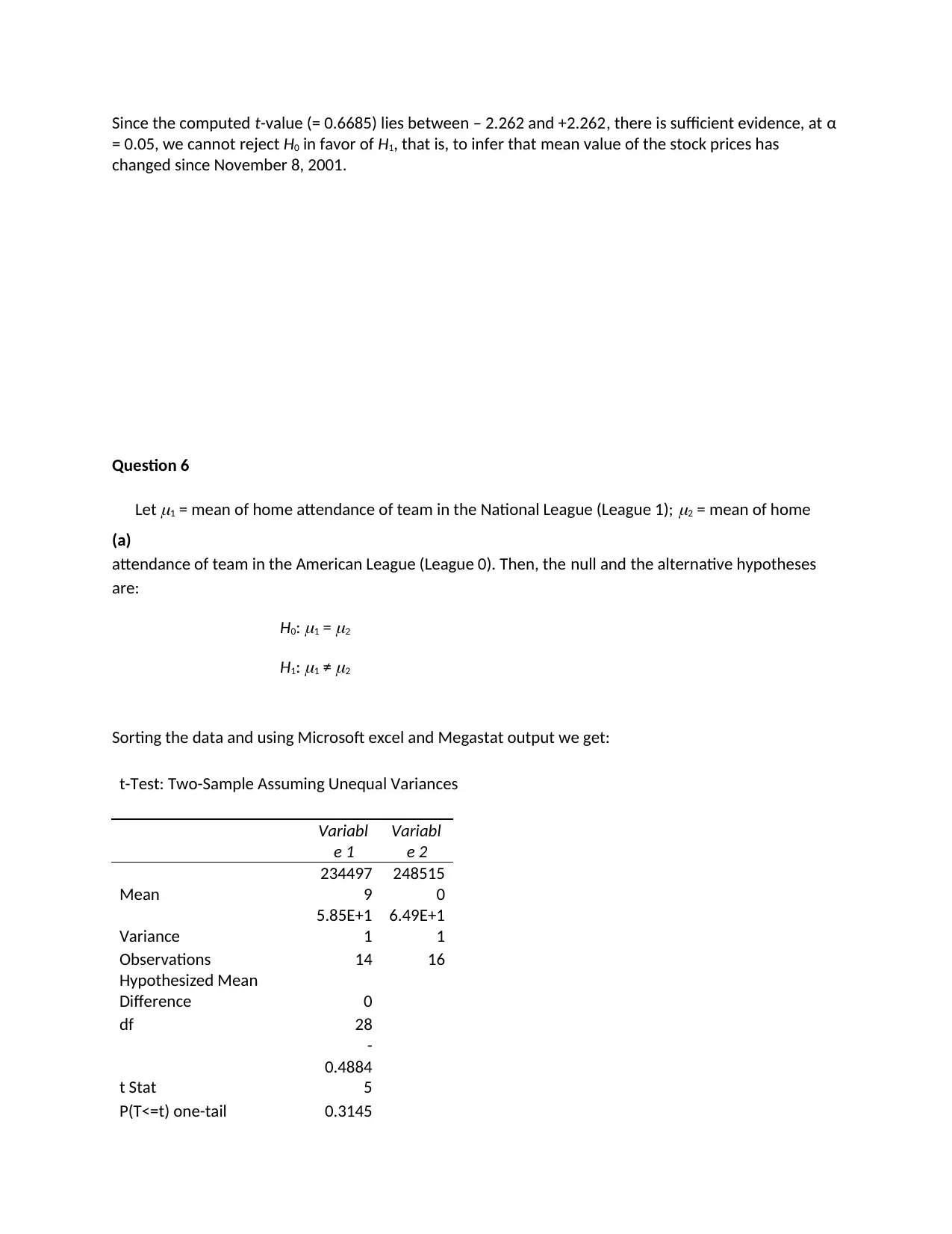
Since the computed t-value (= 0.6685) lies between – 2.262 and +2.262, there is sufficient evidence, at α
= 0.05, we cannot reject H0 in favor of H1, that is, to infer that mean value of the stock prices has
changed since November 8, 2001.
Question 6
(a)
Let
1 = mean of home attendance of team in the National League (League 1);
2 = mean of home
attendance of team in the American League (League 0). Then, the null and the alternative hypotheses
are:
H0:
1 =
2
H1:
1 ≠
2
Sorting the data and using Microsoft excel and Megastat output we get:
t-Test: Two-Sample Assuming Unequal Variances
Variabl
e 1
Variabl
e 2
Mean
234497
9
248515
0
Variance
5.85E+1
1
6.49E+1
1
Observations 14 16
Hypothesized Mean
Difference 0
df 28
t Stat
-
0.4884
5
P(T<=t) one-tail 0.3145

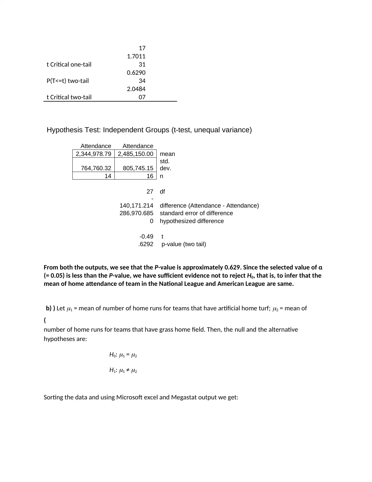
17
t Critical one-tail
1.7011
31
P(T<=t) two-tail
0.6290
34
t Critical two-tail
2.0484
07
Hypothesis Test: Independent Groups (t-test, unequal variance)
Attendance Attendance
2,344,978.79 2,485,150.00 mean
764,760.32 805,745.15
std.
dev.
14 16 n
27 df
-
140,171.214 difference (Attendance - Attendance)
286,970.685 standard error of difference
0 hypothesized difference
-0.49 t
.6292 p-value (two tail)
From both the outputs, we see that the P-value is approximately 0.629. Since the selected value of α
(= 0.05) is less than the P-value, we have sufficient evidence not to reject H0, that is, to infer that the
mean of home attendance of team in the National League and American League are same.
(
b) ) Let
1 = mean of number of home runs for teams that have artificial home turf;
2 = mean of
number of home runs for teams that have grass home field. Then, the null and the alternative
hypotheses are:
H0:
1 =
2
H1:
1 ≠
2
Sorting the data and using Microsoft excel and Megastat output we get:

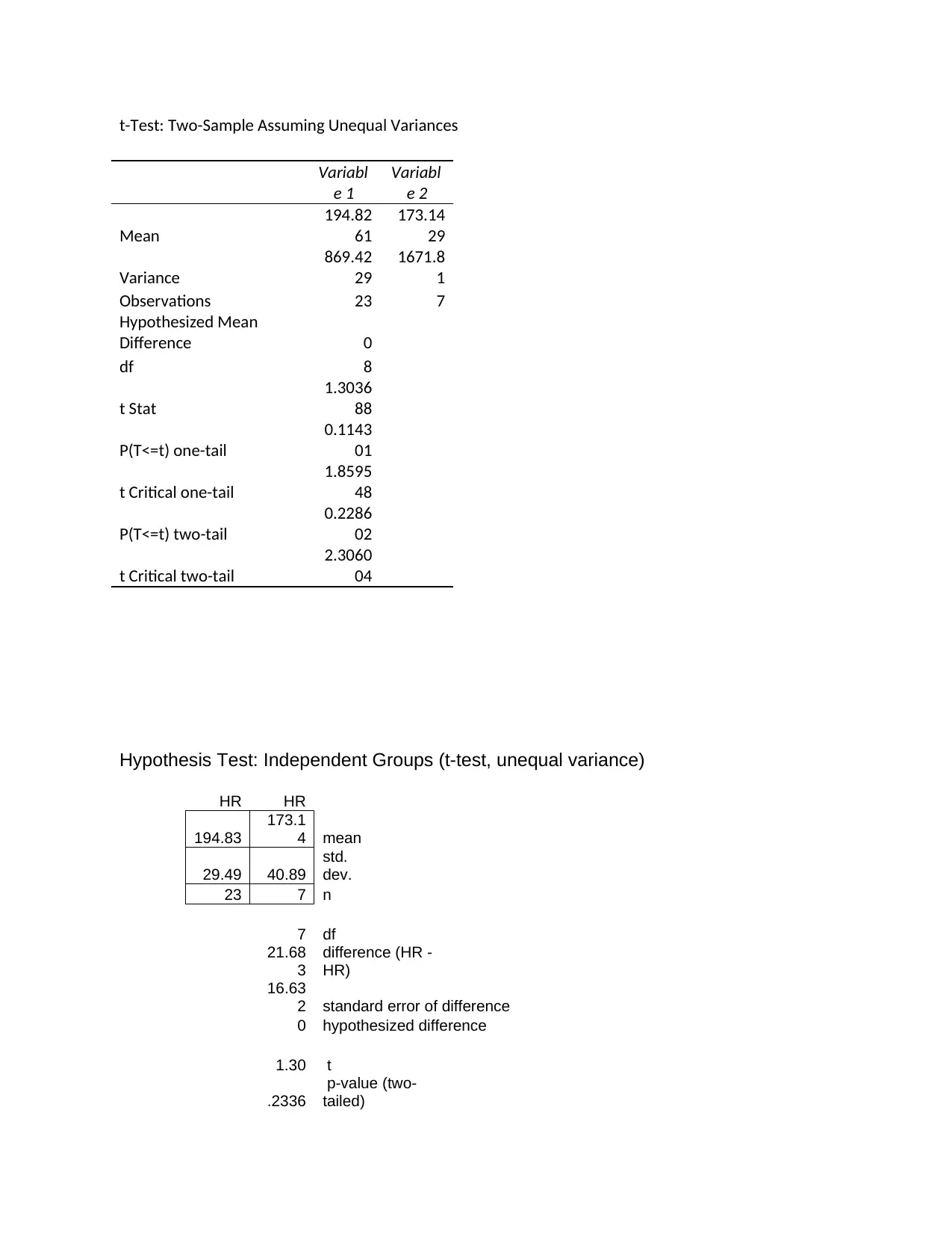
t-Test: Two-Sample Assuming Unequal Variances
Variabl
e 1
Variabl
e 2
Mean
194.82
61
173.14
29
Variance
869.42
29
1671.8
1
Observations 23 7
Hypothesized Mean
Difference 0
df 8
t Stat
1.3036
88
P(T<=t) one-tail
0.1143
01
t Critical one-tail
1.8595
48
P(T<=t) two-tail
0.2286
02
t Critical two-tail
2.3060
04
Hypothesis Test: Independent Groups (t-test, unequal variance)
HR HR
194.83
173.1
4 mean
29.49 40.89
std.
dev.
23 7 n
7 df
21.68
3
difference (HR -
HR)
16.63
2 standard error of difference
0 hypothesized difference
1.30 t
.2336
p-value (two-
tailed)

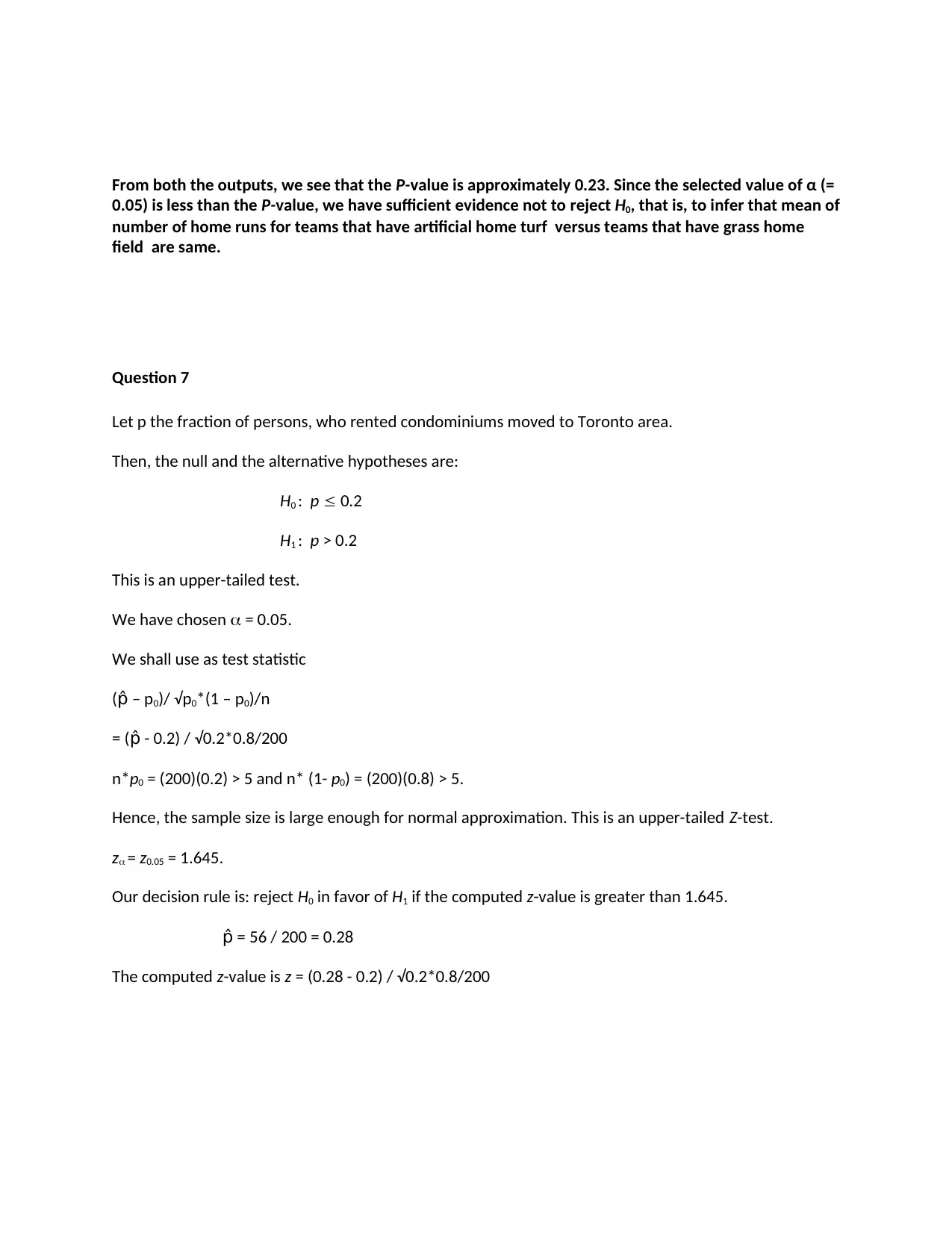
From both the outputs, we see that the P-value is approximately 0.23. Since the selected value of α (=
0.05) is less than the P-value, we have sufficient evidence not to reject H0, that is, to infer that mean of
number of home runs for teams that have artificial home turf versus teams that have grass home
field are same.
Question 7
Let p the fraction of persons, who rented condominiums moved to Toronto area.
Then, the null and the alternative hypotheses are:
H0 : p  0.2
H1 : p > 0.2
This is an upper-tailed test.
We have chosen  = 0.05.
We shall use as test statistic
( – pp̂ 0)/ √p0*(1 – p0)/n
= ( - 0.2) / √0.2*0.8/200p̂
n*p0 = (200)(0.2) > 5 and n* (1- p0) = (200)(0.8) > 5.
Hence, the sample size is large enough for normal approximation. This is an upper-tailed Z-test.
z = z0.05 = 1.645.
Our decision rule is: reject H0 in favor of H1 if the computed z-value is greater than 1.645.
= 56 / 200 = 0.28p̂
The computed z-value is z = (0.28 - 0.2) / √0.2*0.8/200

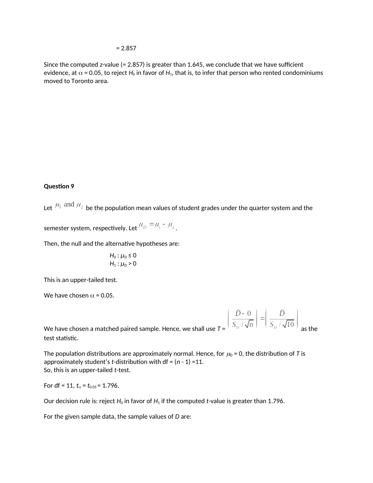
= 2.857
Since the computed z-value (= 2.857) is greater than 1.645, we conclude that we have sufficient
evidence, at  = 0.05, to reject H0 in favor of H1, that is, to infer that person who rented condominiums
moved to Toronto area.
Question 9
Let be the population mean values of student grades under the quarter system and the
semester system, respectively. Let .
Then, the null and the alternative hypotheses are:
H0 : μD ≤ 0
H1 : μD > 0
This is an upper-tailed test.
We have chosen  = 0.05.
We have chosen a matched paired sample. Hence, we shall use T = as the
test statistic.
The population distributions are approximately normal. Hence, for
D = 0, the distribution of T is
approximately student’s t-distribution with df = (n - 1) =11.
So, this is an upper-tailed t-test.
For df = 11, t = t0.05 = 1.796.
Our decision rule is: reject H0 in favor of H1 if the computed t-value is greater than 1.796.
For the given sample data, the sample values of D are:

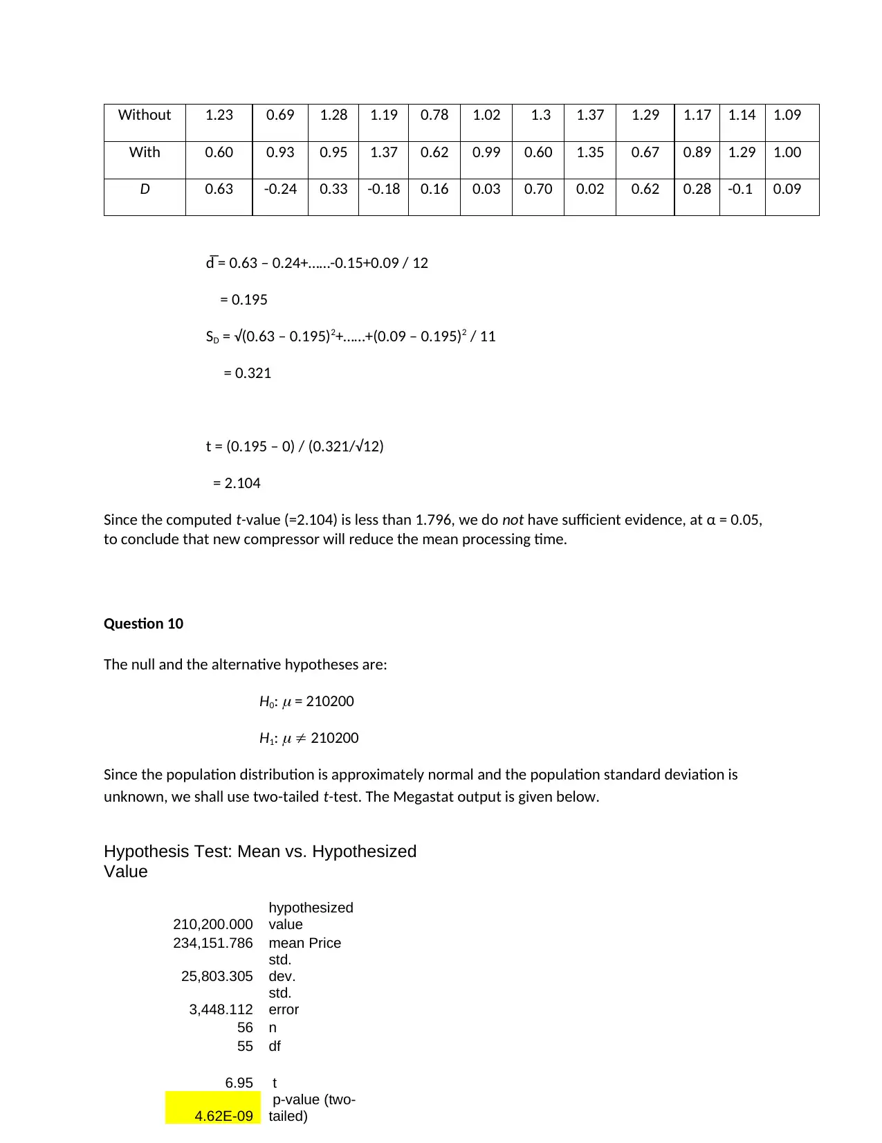
Without 1.23 0.69 1.28 1.19 0.78 1.02 1.3 1.37 1.29 1.17 1.14 1.09
With 0.60 0.93 0.95 1.37 0.62 0.99 0.60 1.35 0.67 0.89 1.29 1.00
D 0.63 -0.24 0.33 -0.18 0.16 0.03 0.70 0.02 0.62 0.28 -0.1 0.09
d̅ = 0.63 – 0.24+……-0.15+0.09 / 12
= 0.195
SD = √(0.63 – 0.195)2+……+(0.09 – 0.195)2 / 11
= 0.321
t = (0.195 – 0) / (0.321/√12)
= 2.104
Since the computed t-value (=2.104) is less than 1.796, we do not have sufficient evidence, at α = 0.05,
to conclude that new compressor will reduce the mean processing time.
Question 10
The null and the alternative hypotheses are:
H0:
 = 210200
H1:
  210200
Since the population distribution is approximately normal and the population standard deviation is
unknown, we shall use two-tailed t-test. The Megastat output is given below.
Hypothesis Test: Mean vs. Hypothesized
Value
210,200.000
hypothesized
value
234,151.786 mean Price
25,803.305
std.
dev.
3,448.112
std.
error
56 n
55 df
6.95 t
4.62E-09
p-value (two-
tailed)

We see from computer output that P-value is a very small quantity. Hence, our conclusion would be “we
have sufficient evidence to reject H0” if the selected  value is greater than the p-value. Since the given
value  = 0.05 > 4.62E-09, we reject H0, that is we infer that the average value of the houses sold in
Victoria during the year 2001 was different from 210200.