Macroeconomics Principles and Applications
VerifiedAdded on 2020/02/24
|24
|3489
|92
AI Summary
This assignment delves into core macroeconomic principles, examining concepts such as real GDP, productive capacity, net social welfare, aggregate demand, and aggregate supply. It analyzes the strengths and weaknesses of each indicator and explores how shifts in these factors can impact an economy's performance. The assignment also discusses the influence of household savings on consumer expenditure and its role in economic recovery from recessions.
Contribute Materials
Your contribution can guide someone’s learning journey. Share your
documents today.
Running head: ECONOMICS OF THE ENVIRONMENT
ECONOMICS OF THE ENIVIRONMENT
Name of the Student
Name of the University
Author’s Note
ECONOMICS OF THE ENIVIRONMENT
Name of the Student
Name of the University
Author’s Note
Secure Best Marks with AI Grader
Need help grading? Try our AI Grader for instant feedback on your assignments.
1ECONOMICS OF THE ENVIRONMENT
Table of Contents
Question 1.1.....................................................................................................................................3
Question 1.2.....................................................................................................................................4
Question 1.3.....................................................................................................................................5
Question 1.4.....................................................................................................................................8
Question 2.1.....................................................................................................................................9
Question 2.2...................................................................................................................................10
Question 2.3...................................................................................................................................10
Question 2.4...................................................................................................................................11
Question 2.5...................................................................................................................................12
Question 3.1...................................................................................................................................14
Question 3.2...................................................................................................................................15
Question 3.3...................................................................................................................................16
Question 3.4...................................................................................................................................16
Question 3.5...................................................................................................................................16
Question 3.6...................................................................................................................................17
Question 3.7...................................................................................................................................22
2ECONOMICS OF THE ENVIRONMENT
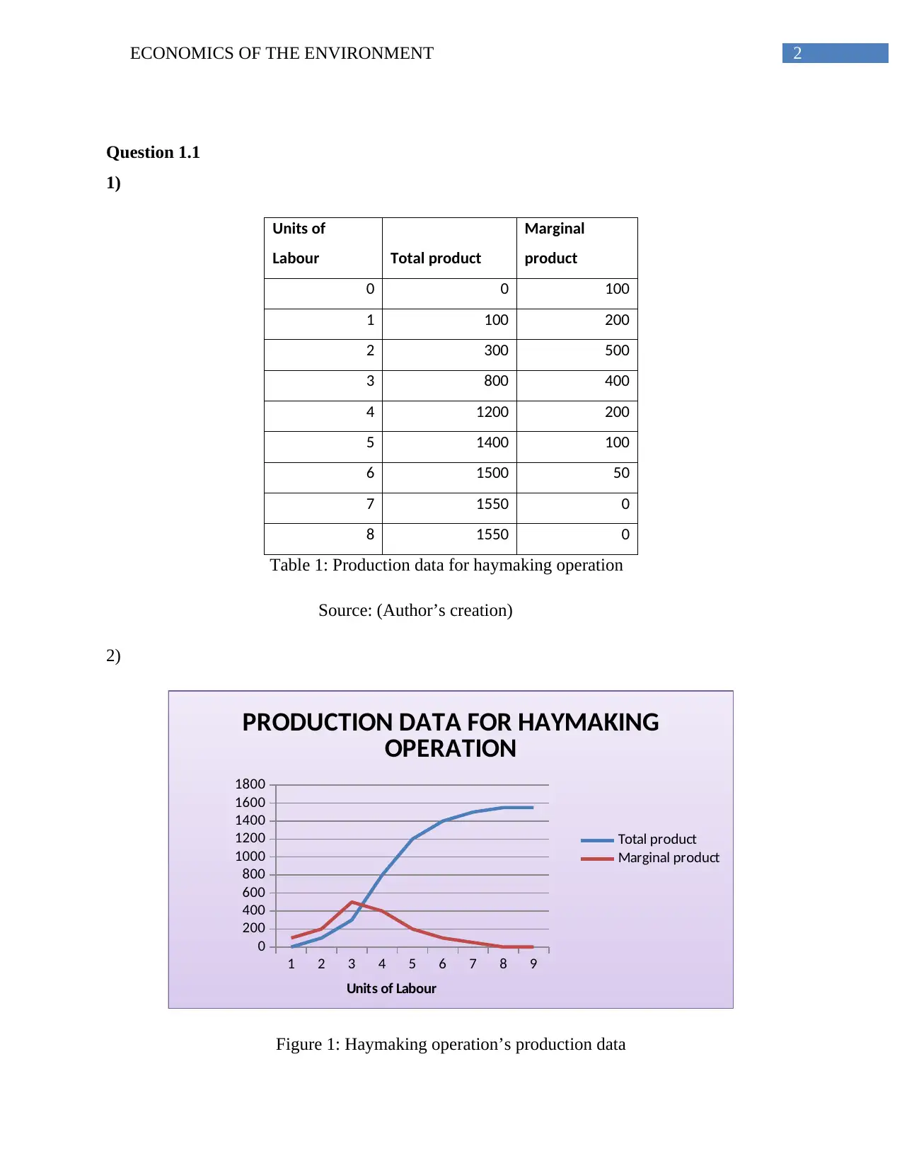
Question 1.1
1)
Units of
Labour Total product
Marginal
product
0 0 100
1 100 200
2 300 500
3 800 400
4 1200 200
5 1400 100
6 1500 50
7 1550 0
8 1550 0
Table 1: Production data for haymaking operation
Source: (Author’s creation)
2)
1 2 3 4 5 6 7 8 9
0
200
400
600
800
1000
1200
1400
1600
1800
PRODUCTION DATA FOR HAYMAKING
OPERATION
Total product
Marginal product
Units of Labour
Figure 1: Haymaking operation’s production data
3ECONOMICS OF THE ENVIRONMENT
Source: (Author’s creation)
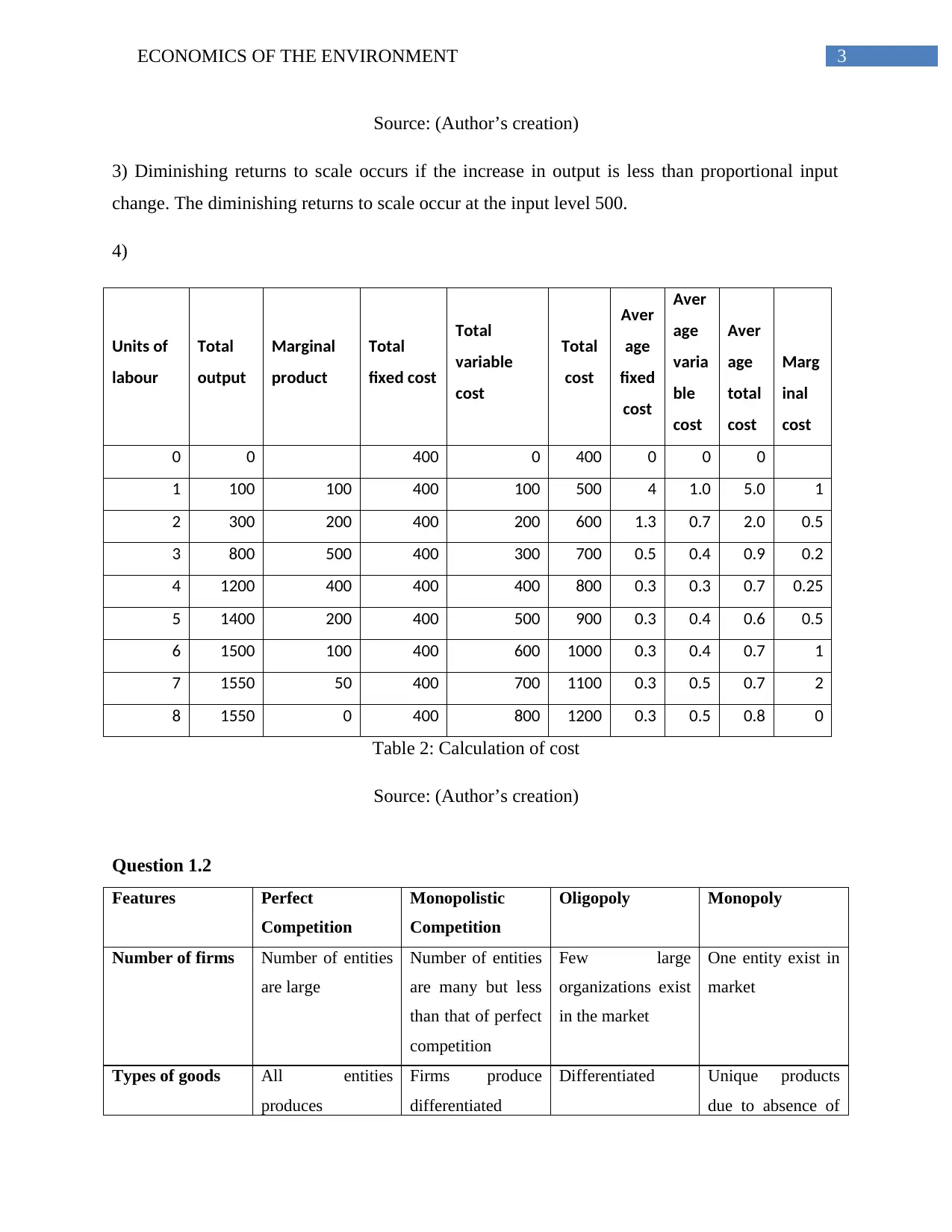
3) Diminishing returns to scale occurs if the increase in output is less than proportional input
change. The diminishing returns to scale occur at the input level 500.
4)
Units of
labour
Total
output
Marginal
product
Total
fixed cost
Total
variable
cost
Total
cost
Aver
age
fixed
cost
Aver
age
varia
ble
cost
Aver
age
total
cost
Marg
inal
cost
0 0 400 0 400 0 0 0
1 100 100 400 100 500 4 1.0 5.0 1
2 300 200 400 200 600 1.3 0.7 2.0 0.5
3 800 500 400 300 700 0.5 0.4 0.9 0.2
4 1200 400 400 400 800 0.3 0.3 0.7 0.25
5 1400 200 400 500 900 0.3 0.4 0.6 0.5
6 1500 100 400 600 1000 0.3 0.4 0.7 1
7 1550 50 400 700 1100 0.3 0.5 0.7 2
8 1550 0 400 800 1200 0.3 0.5 0.8 0
Table 2: Calculation of cost
Source: (Author’s creation)
Question 1.2
Features Perfect
Competition
Monopolistic
Competition
Oligopoly Monopoly
Number of firms Number of entities
are large
Number of entities
are many but less
than that of perfect
competition
Few large
organizations exist
in the market
One entity exist in
market
Types of goods All entities
produces
Firms produce
differentiated
Differentiated Unique products
due to absence of
Source: (Author’s creation)
3) Diminishing returns to scale occurs if the increase in output is less than proportional input
change. The diminishing returns to scale occur at the input level 500.
4)
Units of
labour
Total
output
Marginal
product
Total
fixed cost
Total
variable
cost
Total
cost
Aver
age
fixed
cost
Aver
age
varia
ble
cost
Aver
age
total
cost
Marg
inal
cost
0 0 400 0 400 0 0 0
1 100 100 400 100 500 4 1.0 5.0 1
2 300 200 400 200 600 1.3 0.7 2.0 0.5
3 800 500 400 300 700 0.5 0.4 0.9 0.2
4 1200 400 400 400 800 0.3 0.3 0.7 0.25
5 1400 200 400 500 900 0.3 0.4 0.6 0.5
6 1500 100 400 600 1000 0.3 0.4 0.7 1
7 1550 50 400 700 1100 0.3 0.5 0.7 2
8 1550 0 400 800 1200 0.3 0.5 0.8 0
Table 2: Calculation of cost
Source: (Author’s creation)
Question 1.2
Features Perfect
Competition
Monopolistic
Competition
Oligopoly Monopoly
Number of firms Number of entities
are large
Number of entities
are many but less
than that of perfect
competition
Few large
organizations exist
in the market
One entity exist in
market
Types of goods All entities
produces
Firms produce
differentiated
Differentiated Unique products
due to absence of
Secure Best Marks with AI Grader
Need help grading? Try our AI Grader for instant feedback on your assignments.
4ECONOMICS OF THE ENVIRONMENT
homogeneous
goods
goods goods other firms
Type of price
setting behavior
All entities are
price takers
Entities are price
makers
Entities influence
product prices
Entities are price
maker
Entry conditions No barriers in
firms entrance and
exit
No hurdle in
entrance and exit
Firms face barriers
in entering the
market
Entities face
hurdle in entrance
and exiting the
market
The form of
demand curve
Demand curve for
individual entity is
horizontal
Demand curve is
negatively sloped
Uncertain demand
curve (Kinked
shaped)
Negatively sloped
demand curve
Elasticity of
demand
Perfectly elastic
products
Elasticity of
demand is elevated
but not close to
perfectly elastic
Demand for
commodities is
elastic
Demand for
commodities is
relatively elastic.
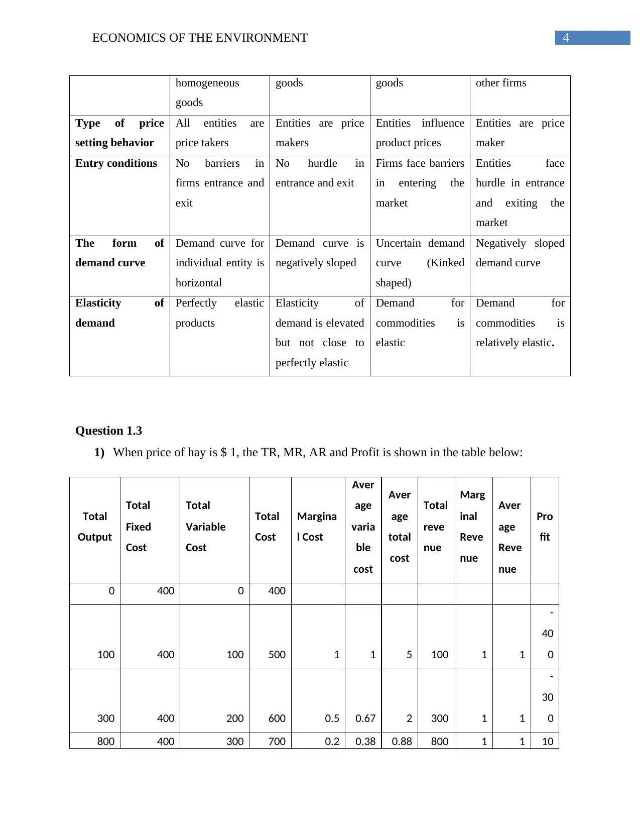
Question 1.3
1) When price of hay is $ 1, the TR, MR, AR and Profit is shown in the table below:
Total
Output
Total
Fixed
Cost
Total
Variable
Cost
Total
Cost
Margina
l Cost
Aver
age
varia
ble
cost
Aver
age
total
cost
Total
reve
nue
Marg
inal
Reve
nue
Aver
age
Reve
nue
Pro
fit
0 400 0 400
100 400 100 500 1 1 5 100 1 1
-
40
0
300 400 200 600 0.5 0.67 2 300 1 1
-
30
0
800 400 300 700 0.2 0.38 0.88 800 1 1 10
homogeneous
goods
goods goods other firms
Type of price
setting behavior
All entities are
price takers
Entities are price
makers
Entities influence
product prices
Entities are price
maker
Entry conditions No barriers in
firms entrance and
exit
No hurdle in
entrance and exit
Firms face barriers
in entering the
market
Entities face
hurdle in entrance
and exiting the
market
The form of
demand curve
Demand curve for
individual entity is
horizontal
Demand curve is
negatively sloped
Uncertain demand
curve (Kinked
shaped)
Negatively sloped
demand curve
Elasticity of
demand
Perfectly elastic
products
Elasticity of
demand is elevated
but not close to
perfectly elastic
Demand for
commodities is
elastic
Demand for
commodities is
relatively elastic.
Question 1.3
1) When price of hay is $ 1, the TR, MR, AR and Profit is shown in the table below:
Total
Output
Total
Fixed
Cost
Total
Variable
Cost
Total
Cost
Margina
l Cost
Aver
age
varia
ble
cost
Aver
age
total
cost
Total
reve
nue
Marg
inal
Reve
nue
Aver
age
Reve
nue
Pro
fit
0 400 0 400
100 400 100 500 1 1 5 100 1 1
-
40
0
300 400 200 600 0.5 0.67 2 300 1 1
-
30
0
800 400 300 700 0.2 0.38 0.88 800 1 1 10
5ECONOMICS OF THE ENVIRONMENT
0
1200 400 400 800 0.25 0.33 0.67 1200 1 1
40
0
1400 400 500 900 0.5 0.36 0.64 1400 1 1
50
0
1500 400 600 1000 1 0.4 0.67 1500 1 1
50
0
1550 400 700 1100 2 0.45 0.71 1550 1 1
45
0
1650 400 800 1200 1 0.5 0.78 1650 1 1
45
0
1700 400 900 1300 2 0.53 0.7 1700 1 1
40
0
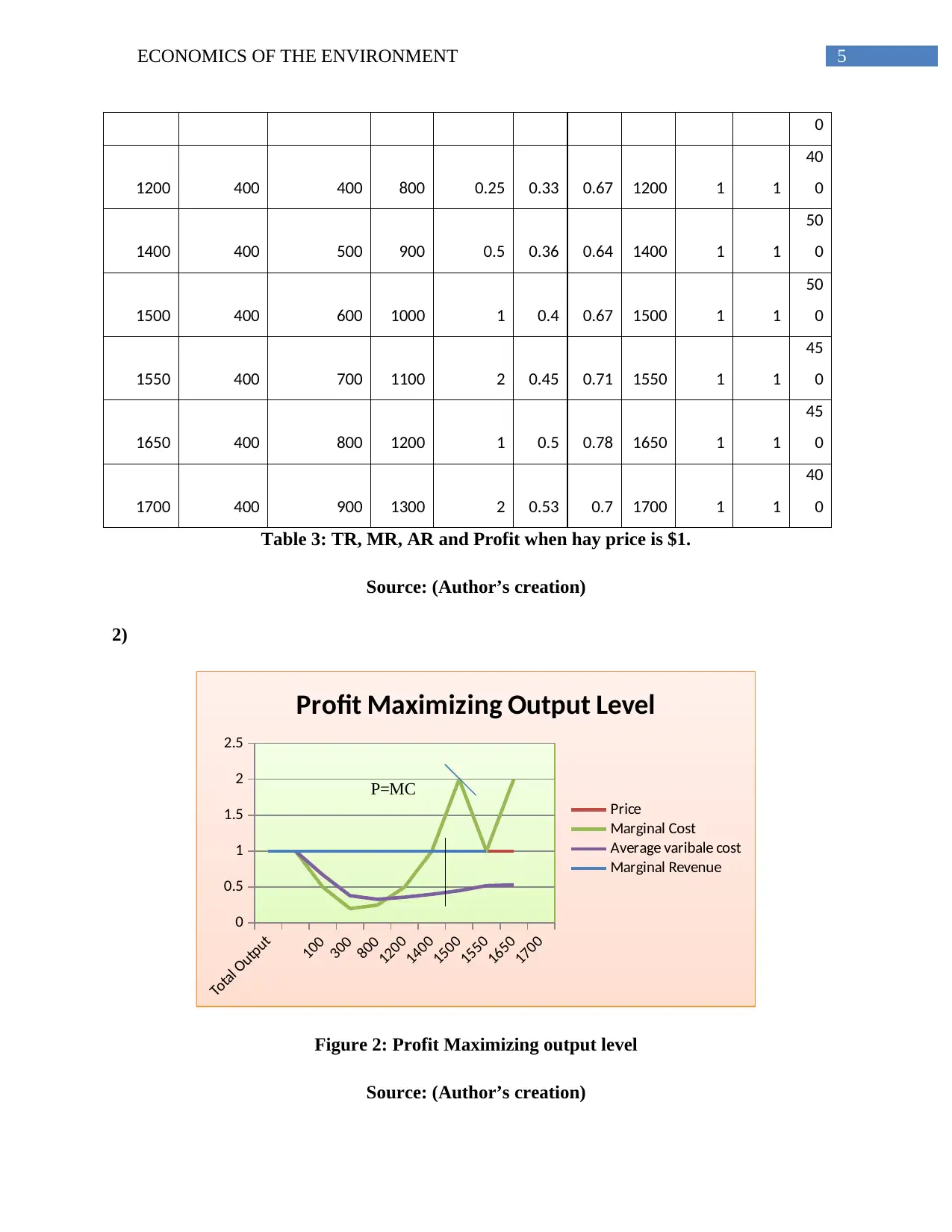
Table 3: TR, MR, AR and Profit when hay price is $1.
Source: (Author’s creation)
2)
Total Output
100
300
800
1200
1400
1500
1550
1650
1700
0
0.5
1
1.5
2
2.5
Profit Maximizing Output Level
Price
Marginal Cost
Average varibale cost
Marginal Revenue
P=MC
Figure 2: Profit Maximizing output level
Source: (Author’s creation)
0
1200 400 400 800 0.25 0.33 0.67 1200 1 1
40
0
1400 400 500 900 0.5 0.36 0.64 1400 1 1
50
0
1500 400 600 1000 1 0.4 0.67 1500 1 1
50
0
1550 400 700 1100 2 0.45 0.71 1550 1 1
45
0
1650 400 800 1200 1 0.5 0.78 1650 1 1
45
0
1700 400 900 1300 2 0.53 0.7 1700 1 1
40
0
Table 3: TR, MR, AR and Profit when hay price is $1.
Source: (Author’s creation)
2)
Total Output
100
300
800
1200
1400
1500
1550
1650
1700
0
0.5
1
1.5
2
2.5
Profit Maximizing Output Level
Price
Marginal Cost
Average varibale cost
Marginal Revenue
P=MC
Figure 2: Profit Maximizing output level
Source: (Author’s creation)
6ECONOMICS OF THE ENVIRONMENT
The above figure shows that price and marginal revenue curve is a horizontal line as it is
constant at all output levels. The marginal cost curve (MR=P) cuts from below and profit
maximizing output level occurs when MC intersects price curve (P=MC) at perfect competition
(Hall and Lieberman, 2012). However, this situation lies between the output levels 1400, where
profit is $500.
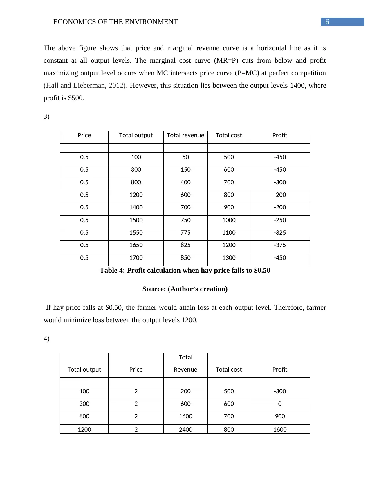
3)
Price Total output Total revenue Total cost Profit
0.5 100 50 500 -450
0.5 300 150 600 -450
0.5 800 400 700 -300
0.5 1200 600 800 -200
0.5 1400 700 900 -200
0.5 1500 750 1000 -250
0.5 1550 775 1100 -325
0.5 1650 825 1200 -375
0.5 1700 850 1300 -450
Table 4: Profit calculation when hay price falls to $0.50
Source: (Author’s creation)
If hay price falls at $0.50, the farmer would attain loss at each output level. Therefore, farmer
would minimize loss between the output levels 1200.
4)
Total output Price
Total
Revenue Total cost Profit
100 2 200 500 -300
300 2 600 600 0
800 2 1600 700 900
1200 2 2400 800 1600
The above figure shows that price and marginal revenue curve is a horizontal line as it is
constant at all output levels. The marginal cost curve (MR=P) cuts from below and profit
maximizing output level occurs when MC intersects price curve (P=MC) at perfect competition
(Hall and Lieberman, 2012). However, this situation lies between the output levels 1400, where
profit is $500.
3)
Price Total output Total revenue Total cost Profit
0.5 100 50 500 -450
0.5 300 150 600 -450
0.5 800 400 700 -300
0.5 1200 600 800 -200
0.5 1400 700 900 -200
0.5 1500 750 1000 -250
0.5 1550 775 1100 -325
0.5 1650 825 1200 -375
0.5 1700 850 1300 -450
Table 4: Profit calculation when hay price falls to $0.50
Source: (Author’s creation)
If hay price falls at $0.50, the farmer would attain loss at each output level. Therefore, farmer
would minimize loss between the output levels 1200.
4)
Total output Price
Total
Revenue Total cost Profit
100 2 200 500 -300
300 2 600 600 0
800 2 1600 700 900
1200 2 2400 800 1600
Paraphrase This Document
Need a fresh take? Get an instant paraphrase of this document with our AI Paraphraser
7ECONOMICS OF THE ENVIRONMENT
1400 2 2800 900 1900
1500 2 3000 1000 2000
1550 2 3100 1100 2000
1650 2 3300 1200 2100
1700 2 3400 1300 2100
Table 5: Profit of farm when price rise to $2
Source: (Author’s creation)
If the price of hay rises to $2.00, the profit maximizing level occurs at output level 1650. The
amount of profit at this level is $2100.
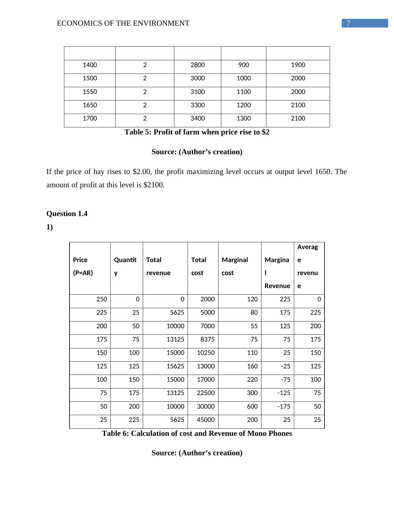
Question 1.4
1)
Price
(P=AR)
Quantit
y
Total
revenue
Total
cost
Marginal
cost
Margina
l
Revenue
Averag
e
revenu
e
250 0 0 2000 120 225 0
225 25 5625 5000 80 175 225
200 50 10000 7000 55 125 200
175 75 13125 8375 75 75 175
150 100 15000 10250 110 25 150
125 125 15625 13000 160 -25 125
100 150 15000 17000 220 -75 100
75 175 13125 22500 300 -125 75
50 200 10000 30000 600 -175 50
25 225 5625 45000 200 25 25
Table 6: Calculation of cost and Revenue of Mono Phones
Source: (Author’s creation)
1400 2 2800 900 1900
1500 2 3000 1000 2000
1550 2 3100 1100 2000
1650 2 3300 1200 2100
1700 2 3400 1300 2100
Table 5: Profit of farm when price rise to $2
Source: (Author’s creation)
If the price of hay rises to $2.00, the profit maximizing level occurs at output level 1650. The
amount of profit at this level is $2100.
Question 1.4
1)
Price
(P=AR)
Quantit
y
Total
revenue
Total
cost
Marginal
cost
Margina
l
Revenue
Averag
e
revenu
e
250 0 0 2000 120 225 0
225 25 5625 5000 80 175 225
200 50 10000 7000 55 125 200
175 75 13125 8375 75 75 175
150 100 15000 10250 110 25 150
125 125 15625 13000 160 -25 125
100 150 15000 17000 220 -75 100
75 175 13125 22500 300 -125 75
50 200 10000 30000 600 -175 50
25 225 5625 45000 200 25 25
Table 6: Calculation of cost and Revenue of Mono Phones
Source: (Author’s creation)
8ECONOMICS OF THE ENVIRONMENT
2)
0 25 50 75 100 125 150 175 200 225
-300
-200
-100
0
100
200
300
400
500
600
700
AR, MR AND MC CURVE
Marginal cost
Marginal Revenue
Average revenue
Total Quantity
MR=M
C
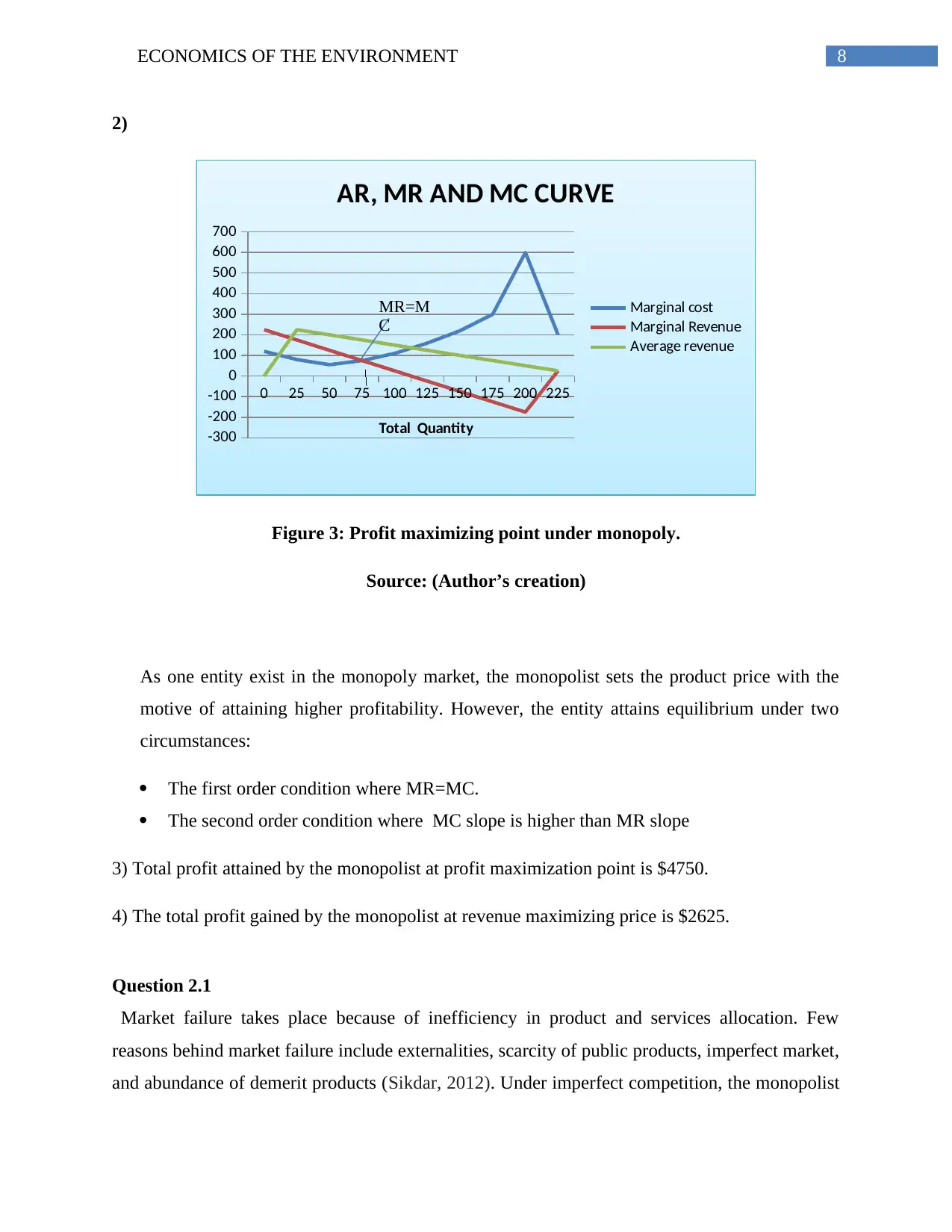
Figure 3: Profit maximizing point under monopoly.
Source: (Author’s creation)
As one entity exist in the monopoly market, the monopolist sets the product price with the
motive of attaining higher profitability. However, the entity attains equilibrium under two
circumstances:
The first order condition where MR=MC.
The second order condition where MC slope is higher than MR slope
3) Total profit attained by the monopolist at profit maximization point is $4750.
4) The total profit gained by the monopolist at revenue maximizing price is $2625.
Question 2.1
Market failure takes place because of inefficiency in product and services allocation. Few
reasons behind market failure include externalities, scarcity of public products, imperfect market,
and abundance of demerit products (Sikdar, 2012). Under imperfect competition, the monopolist
2)
0 25 50 75 100 125 150 175 200 225
-300
-200
-100
0
100
200
300
400
500
600
700
AR, MR AND MC CURVE
Marginal cost
Marginal Revenue
Average revenue
Total Quantity
MR=M
C
Figure 3: Profit maximizing point under monopoly.
Source: (Author’s creation)
As one entity exist in the monopoly market, the monopolist sets the product price with the
motive of attaining higher profitability. However, the entity attains equilibrium under two
circumstances:
The first order condition where MR=MC.
The second order condition where MC slope is higher than MR slope
3) Total profit attained by the monopolist at profit maximization point is $4750.
4) The total profit gained by the monopolist at revenue maximizing price is $2625.
Question 2.1
Market failure takes place because of inefficiency in product and services allocation. Few
reasons behind market failure include externalities, scarcity of public products, imperfect market,
and abundance of demerit products (Sikdar, 2012). Under imperfect competition, the monopolist
9ECONOMICS OF THE ENVIRONMENT
can restrict supply of goods and can create deadweight loss in the respective economy.
Therefore, market failure arises owing to under provision of products. Hence, imperfect markets
curbs output for maximizing profit and this creates failure in market.
Question 2.2
1) Councils flood production systems is considered as public good because of non- excludability
and non- rivalry. Non- excludability means that the people in the respective country are protected
irrespective of their contribution towards cost. Non-rivalry indicates if the country is protected
from increasing flood, it does not decrease the safety provided by the flood production system
for other nation.
2)Pedestrians are considered as free rider because they take benefits of using road safety sign for
slowing down traffic outside school without paying taxes for utilizing road as public goods.
Question 2.3
1) If a school introduces dragon boat racing and kappa haka program for benefitting young
people on academic studies, then it is considered as positive externality that leads to market
failure. Positive externality means positive spillover occurring from these activities will directly
influence the students in school (Rios et al., 2013). Therefore, introduction of this program will
refresh the students mind and this will increase their concentration in academic studies.
Theses cultural activities will motivate the students in winning the competition and receiving
certificates. After they leave the school, this certificate will help the students in showing their
skills in colleges or other job interviews.
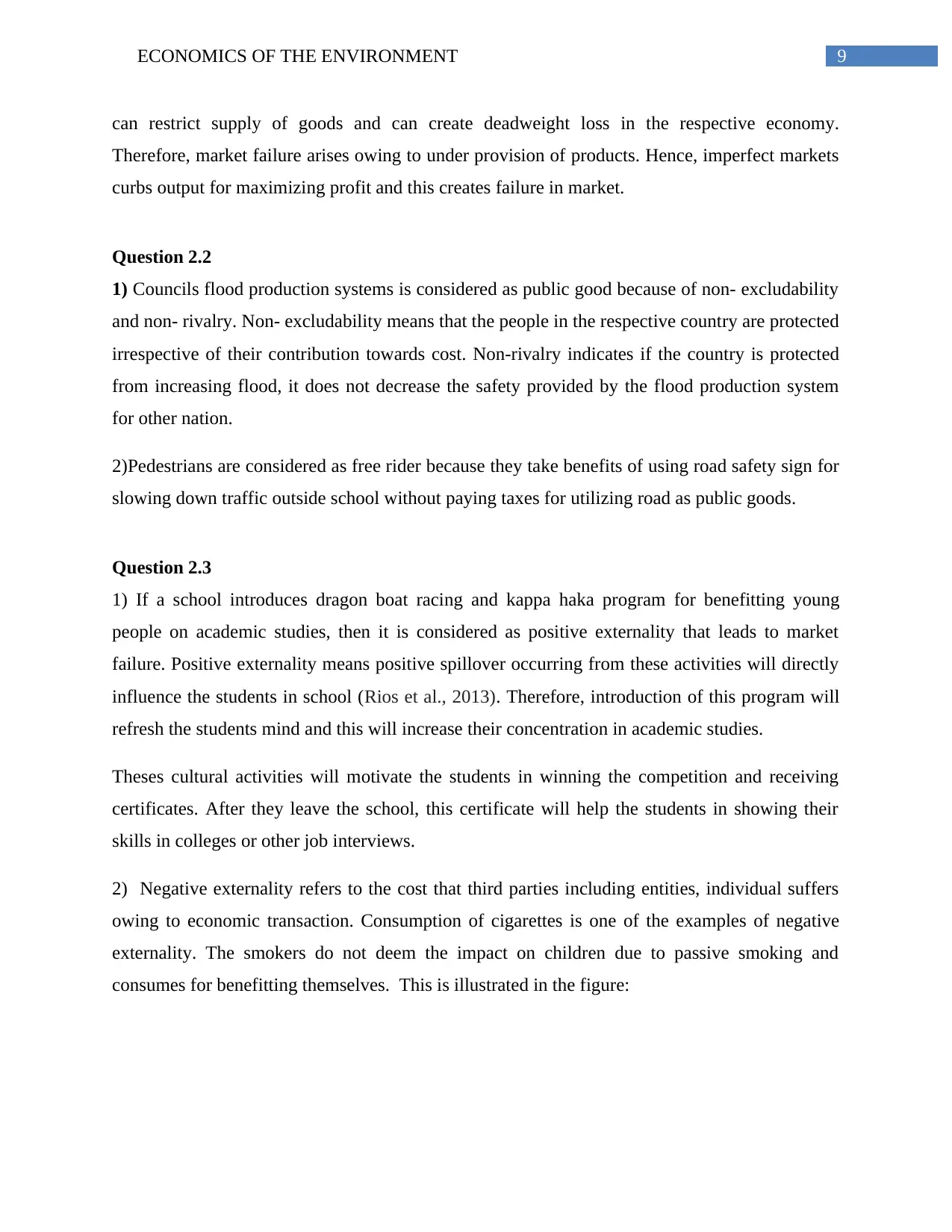
2) Negative externality refers to the cost that third parties including entities, individual suffers
owing to economic transaction. Consumption of cigarettes is one of the examples of negative
externality. The smokers do not deem the impact on children due to passive smoking and
consumes for benefitting themselves. This is illustrated in the figure:
can restrict supply of goods and can create deadweight loss in the respective economy.
Therefore, market failure arises owing to under provision of products. Hence, imperfect markets
curbs output for maximizing profit and this creates failure in market.
Question 2.2
1) Councils flood production systems is considered as public good because of non- excludability
and non- rivalry. Non- excludability means that the people in the respective country are protected
irrespective of their contribution towards cost. Non-rivalry indicates if the country is protected
from increasing flood, it does not decrease the safety provided by the flood production system
for other nation.
2)Pedestrians are considered as free rider because they take benefits of using road safety sign for
slowing down traffic outside school without paying taxes for utilizing road as public goods.
Question 2.3
1) If a school introduces dragon boat racing and kappa haka program for benefitting young
people on academic studies, then it is considered as positive externality that leads to market
failure. Positive externality means positive spillover occurring from these activities will directly
influence the students in school (Rios et al., 2013). Therefore, introduction of this program will
refresh the students mind and this will increase their concentration in academic studies.
Theses cultural activities will motivate the students in winning the competition and receiving
certificates. After they leave the school, this certificate will help the students in showing their
skills in colleges or other job interviews.
2) Negative externality refers to the cost that third parties including entities, individual suffers
owing to economic transaction. Consumption of cigarettes is one of the examples of negative
externality. The smokers do not deem the impact on children due to passive smoking and
consumes for benefitting themselves. This is illustrated in the figure:
Secure Best Marks with AI Grader
Need help grading? Try our AI Grader for instant feedback on your assignments.
10ECONOMICS OF THE ENVIRONMENT
P1
P*
Q* Q1
MSC
MPBMSB
Negative externality
EXEXTERNALITY
Welfare loss
Quantity of cigarettes
Cigarettes price
Figure 4: Smoking as negative externalities
Source: (Author’s creation)
The government adopts policy measures for internalizing negative externalities of cigarettes
smoking that includes:
Banning promotion of tobacco and restricts smoking in all public places.
Increasing tax on tobacco
Introducing campaigns for health education
Question 2.4
It is acceptable that New Zealand’s government must implement excise tax on tobacco products
because it is considered as one of the effective means of decreasing health hazards. Moreover, as
tobacco is luxury goods, shortage in tobacco production will not affect other people and less
demand for tobacco will hardly influence national income of New Zealand (McDowell and Nash,
2012). On the contrary, decline in intake of those products that leads to obesity will affect the
people in the country as it is a necessity goods. Therefore, if the government of New Zealand
11ECONOMICS OF THE ENVIRONMENT
Schooling Years
Cost and Benefits Demand curve
Change in supply curve
Initial supply curve
I
D
L
J
K
H
NM
implements fat tax on these products, then consumption of these products will decline. As a
result, the products supply will reduce and this will influence the country’s total income.
2) Four measures that the government of New Zealand must impose for discouraging eating of
fatty products and promoting healthier goods includes-
Interpretive labeling on the package of fatty products
Marketing regulation to children
Increasing saturated at and beverage tax on sugary goods
Removing GST from healthier foods
Question 2.5
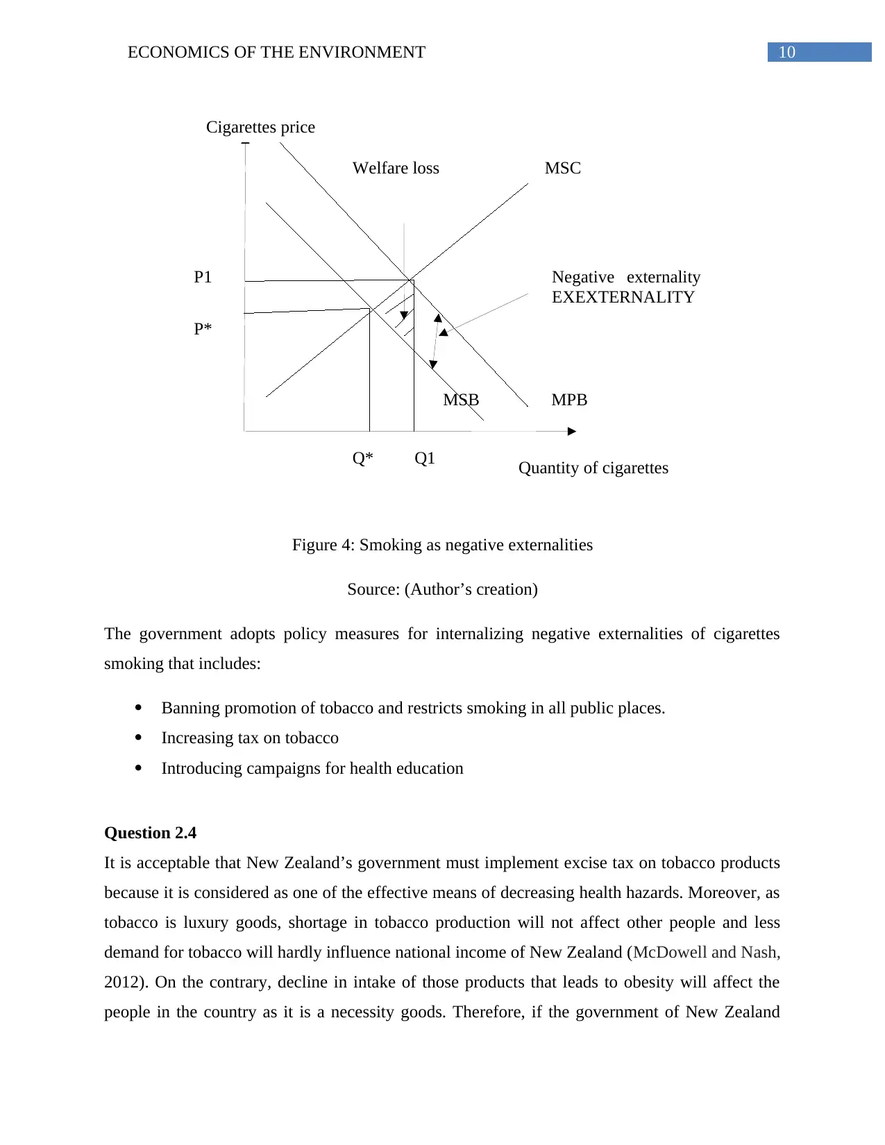
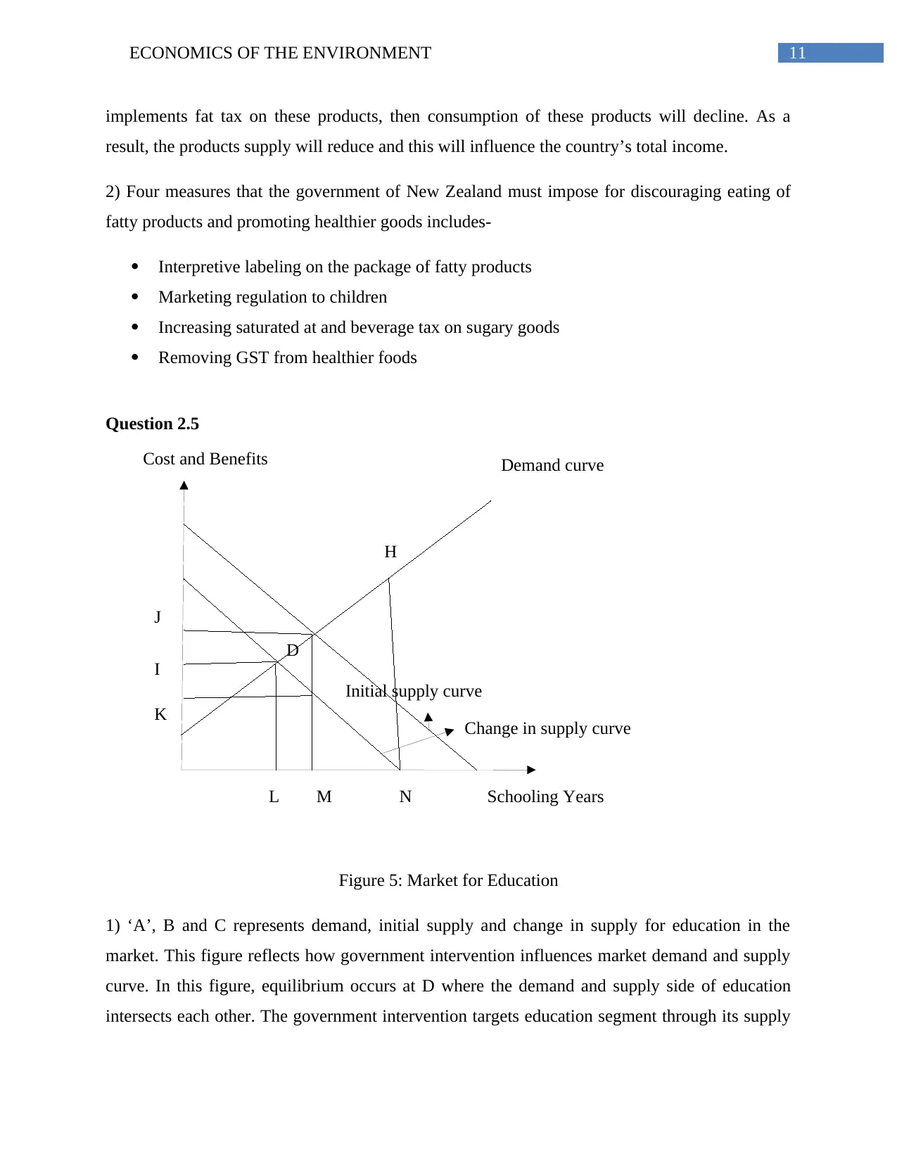
Figure 5: Market for Education
1) ‘A’, B and C represents demand, initial supply and change in supply for education in the
market. This figure reflects how government intervention influences market demand and supply
curve. In this figure, equilibrium occurs at D where the demand and supply side of education
intersects each other. The government intervention targets education segment through its supply
Schooling Years
Cost and Benefits Demand curve
Change in supply curve
Initial supply curve
I
D
L
J
K
H
NM
implements fat tax on these products, then consumption of these products will decline. As a
result, the products supply will reduce and this will influence the country’s total income.
2) Four measures that the government of New Zealand must impose for discouraging eating of
fatty products and promoting healthier goods includes-
Interpretive labeling on the package of fatty products
Marketing regulation to children
Increasing saturated at and beverage tax on sugary goods
Removing GST from healthier foods
Question 2.5
Figure 5: Market for Education
1) ‘A’, B and C represents demand, initial supply and change in supply for education in the
market. This figure reflects how government intervention influences market demand and supply
curve. In this figure, equilibrium occurs at D where the demand and supply side of education
intersects each other. The government intervention targets education segment through its supply
12ECONOMICS OF THE ENVIRONMENT
Q
P
P
Q Q1
Consumers benefit
Producers benefit
P1
side while inadequate attention is paid on its demand side. However, this shifts the supply curve
to left as denoted by C.
2) The education sector in unregulated market basically encompasses of development of skills
including vocational courses and its support services including corporate learning, tutoring
(Caragata, 2012). On the other hand, education sector in regulated market involves government’s
role in protecting children, accrediting schools and free information flow.
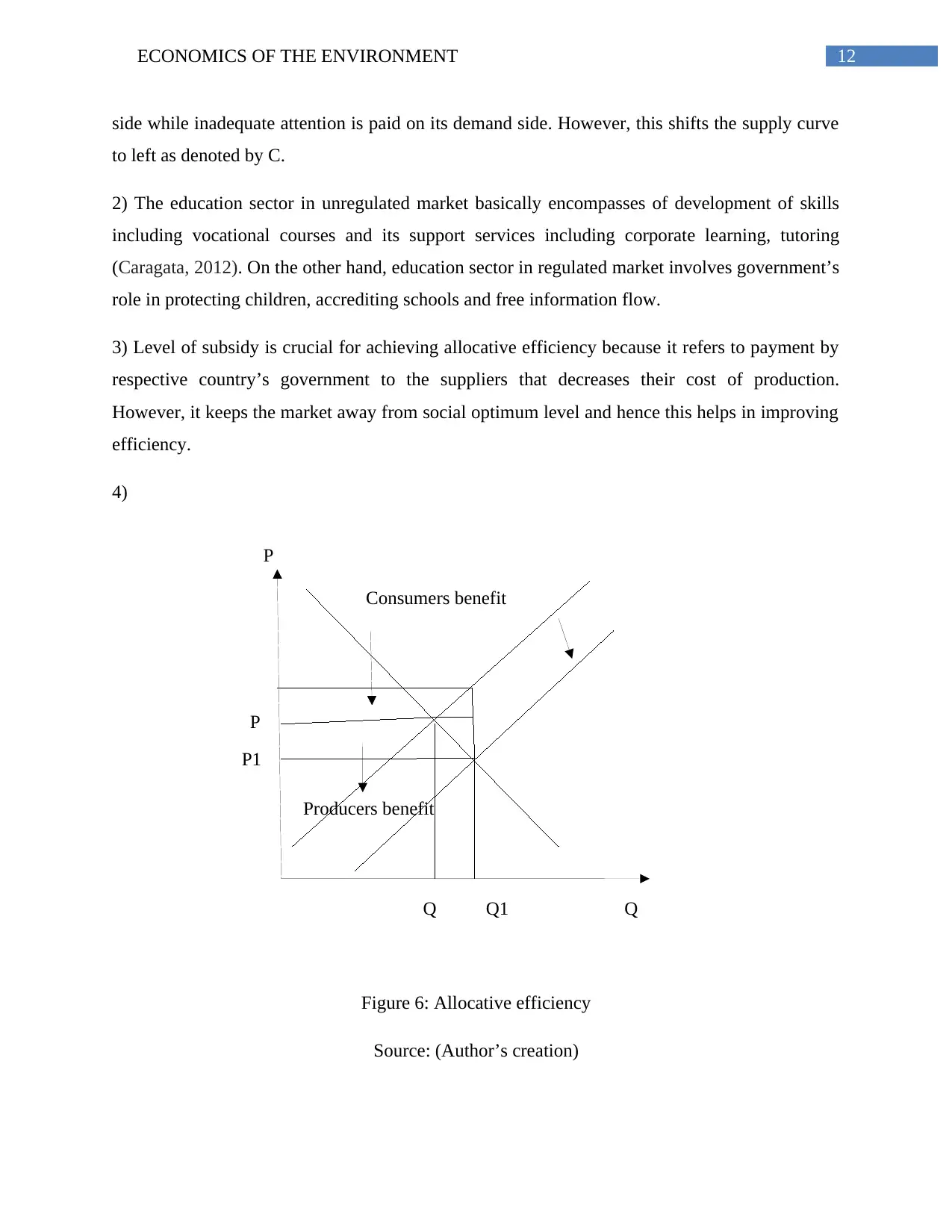
3) Level of subsidy is crucial for achieving allocative efficiency because it refers to payment by
respective country’s government to the suppliers that decreases their cost of production.
However, it keeps the market away from social optimum level and hence this helps in improving
efficiency.
4)
Figure 6: Allocative efficiency
Source: (Author’s creation)
Q
P
P
Q Q1
Consumers benefit
Producers benefit
P1
side while inadequate attention is paid on its demand side. However, this shifts the supply curve
to left as denoted by C.
2) The education sector in unregulated market basically encompasses of development of skills
including vocational courses and its support services including corporate learning, tutoring
(Caragata, 2012). On the other hand, education sector in regulated market involves government’s
role in protecting children, accrediting schools and free information flow.
3) Level of subsidy is crucial for achieving allocative efficiency because it refers to payment by
respective country’s government to the suppliers that decreases their cost of production.
However, it keeps the market away from social optimum level and hence this helps in improving
efficiency.
4)
Figure 6: Allocative efficiency
Source: (Author’s creation)
Paraphrase This Document
Need a fresh take? Get an instant paraphrase of this document with our AI Paraphraser
13ECONOMICS OF THE ENVIRONMENT
Savings
Financial sector
Investmenty Overseas
Exports Imports
Household Government Producers
Monetary Flow
Monetary flow
Subsidies
Taxes
Taxes
Transfer payments
5) Tradeoff between allocative efficiency and equity exists when the given market activity
increases efficiency in productivity and declines distributive equity. It revolves around
transaction cost and involuntary redistribution that prevents the people from attaining maximum
production efficiency.
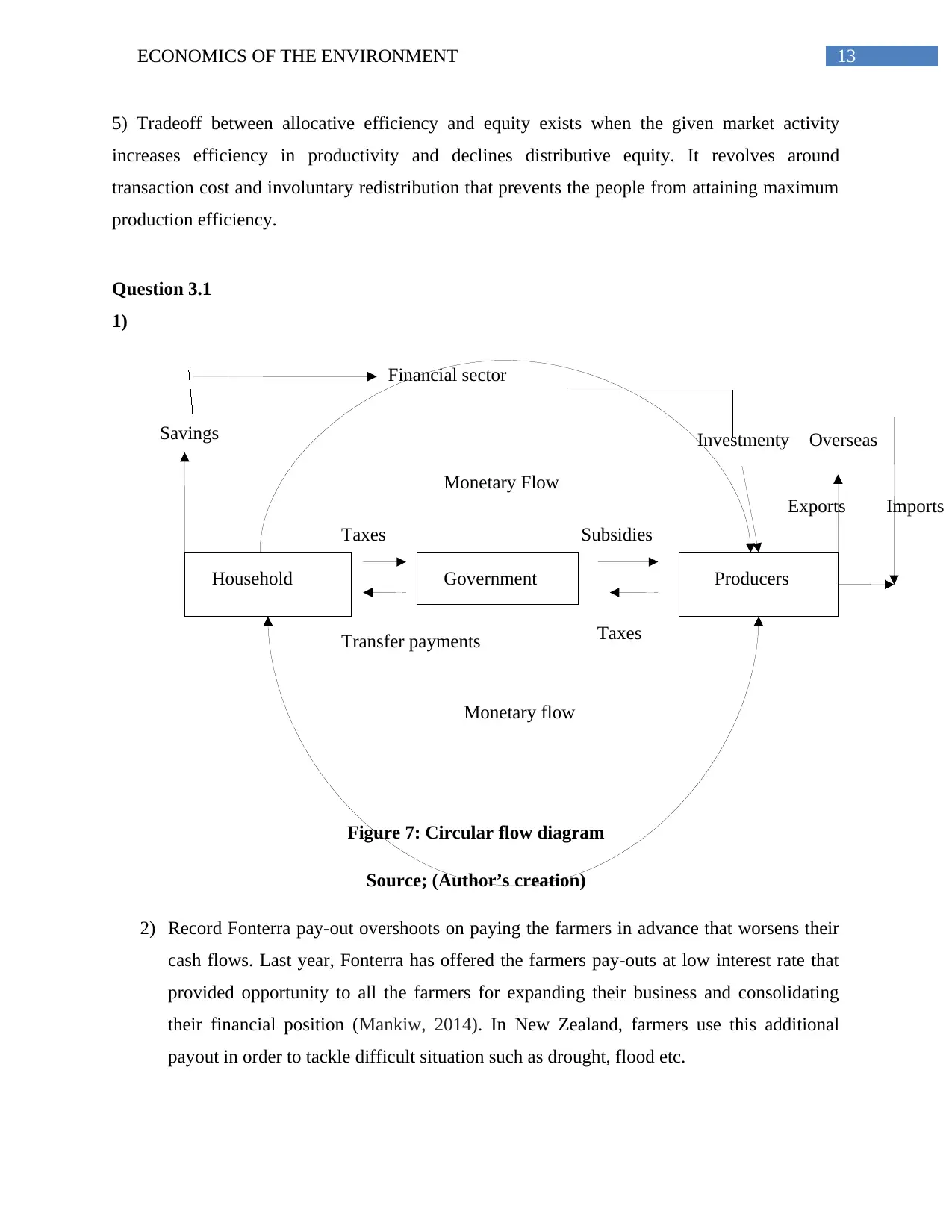
Question 3.1
1)
Figure 7: Circular flow diagram
Source; (Author’s creation)
2) Record Fonterra pay-out overshoots on paying the farmers in advance that worsens their
cash flows. Last year, Fonterra has offered the farmers pay-outs at low interest rate that
provided opportunity to all the farmers for expanding their business and consolidating
their financial position (Mankiw, 2014). In New Zealand, farmers use this additional
payout in order to tackle difficult situation such as drought, flood etc.
Savings
Financial sector
Investmenty Overseas
Exports Imports
Household Government Producers
Monetary Flow
Monetary flow
Subsidies
Taxes
Taxes
Transfer payments
5) Tradeoff between allocative efficiency and equity exists when the given market activity
increases efficiency in productivity and declines distributive equity. It revolves around
transaction cost and involuntary redistribution that prevents the people from attaining maximum
production efficiency.
Question 3.1
1)
Figure 7: Circular flow diagram
Source; (Author’s creation)
2) Record Fonterra pay-out overshoots on paying the farmers in advance that worsens their
cash flows. Last year, Fonterra has offered the farmers pay-outs at low interest rate that
provided opportunity to all the farmers for expanding their business and consolidating
their financial position (Mankiw, 2014). In New Zealand, farmers use this additional
payout in order to tackle difficult situation such as drought, flood etc.
14ECONOMICS OF THE ENVIRONMENT
3) Due this high pay-out, the farmers in New Zealand produces more goods that influences
other manufacturers. As the supply of products improves, the producers try to lower the
product price and this increases the consumers demand for commodities (Tinkler and
Woods, 2013). However, other producers attain higher profitability owing to increase in
product demand.
4) This flow on impact on farmer’s payout directly influences the government of New
Zealand. The government concentrates on providing extra value to the farmers through
various promotions of products (Fry, 2014). This policy helps the farmers to sell their
goods to many retailers that leads to increase in farmers profitability. This also benefits
the policymakers in reducing their subsidies on the farmers.
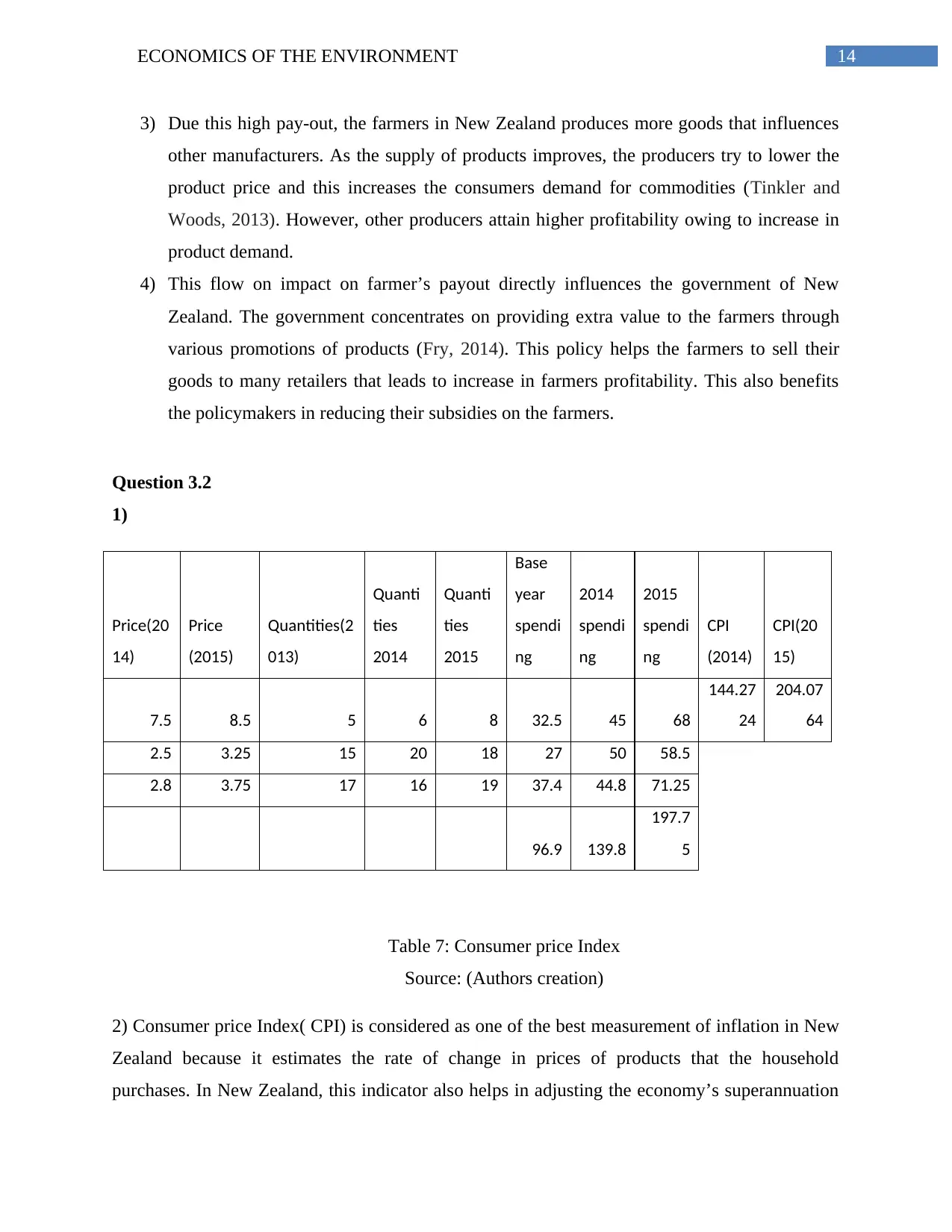
Question 3.2
1)
Price(20
14)
Price
(2015)
Quantities(2
013)
Quanti
ties
2014
Quanti
ties
2015
Base
year
spendi
ng
2014
spendi
ng
2015
spendi
ng
CPI
(2014)
CPI(20
15)
7.5 8.5 5 6 8 32.5 45 68
144.27
24
204.07
64
2.5 3.25 15 20 18 27 50 58.5
2.8 3.75 17 16 19 37.4 44.8 71.25
96.9 139.8
197.7
5
Table 7: Consumer price Index
Source: (Authors creation)
2) Consumer price Index( CPI) is considered as one of the best measurement of inflation in New
Zealand because it estimates the rate of change in prices of products that the household
purchases. In New Zealand, this indicator also helps in adjusting the economy’s superannuation
3) Due this high pay-out, the farmers in New Zealand produces more goods that influences
other manufacturers. As the supply of products improves, the producers try to lower the
product price and this increases the consumers demand for commodities (Tinkler and
Woods, 2013). However, other producers attain higher profitability owing to increase in
product demand.
4) This flow on impact on farmer’s payout directly influences the government of New
Zealand. The government concentrates on providing extra value to the farmers through
various promotions of products (Fry, 2014). This policy helps the farmers to sell their
goods to many retailers that leads to increase in farmers profitability. This also benefits
the policymakers in reducing their subsidies on the farmers.
Question 3.2
1)
Price(20
14)
Price
(2015)
Quantities(2
013)
Quanti
ties
2014
Quanti
ties
2015
Base
year
spendi
ng
2014
spendi
ng
2015
spendi
ng
CPI
(2014)
CPI(20
15)
7.5 8.5 5 6 8 32.5 45 68
144.27
24
204.07
64
2.5 3.25 15 20 18 27 50 58.5
2.8 3.75 17 16 19 37.4 44.8 71.25
96.9 139.8
197.7
5
Table 7: Consumer price Index
Source: (Authors creation)
2) Consumer price Index( CPI) is considered as one of the best measurement of inflation in New
Zealand because it estimates the rate of change in prices of products that the household
purchases. In New Zealand, this indicator also helps in adjusting the economy’s superannuation
15ECONOMICS OF THE ENVIRONMENT
and benefit payments of unemployment every year. Moreover, it also indicates in ensuring that
payments have maintained the consumer’s purchasing power.
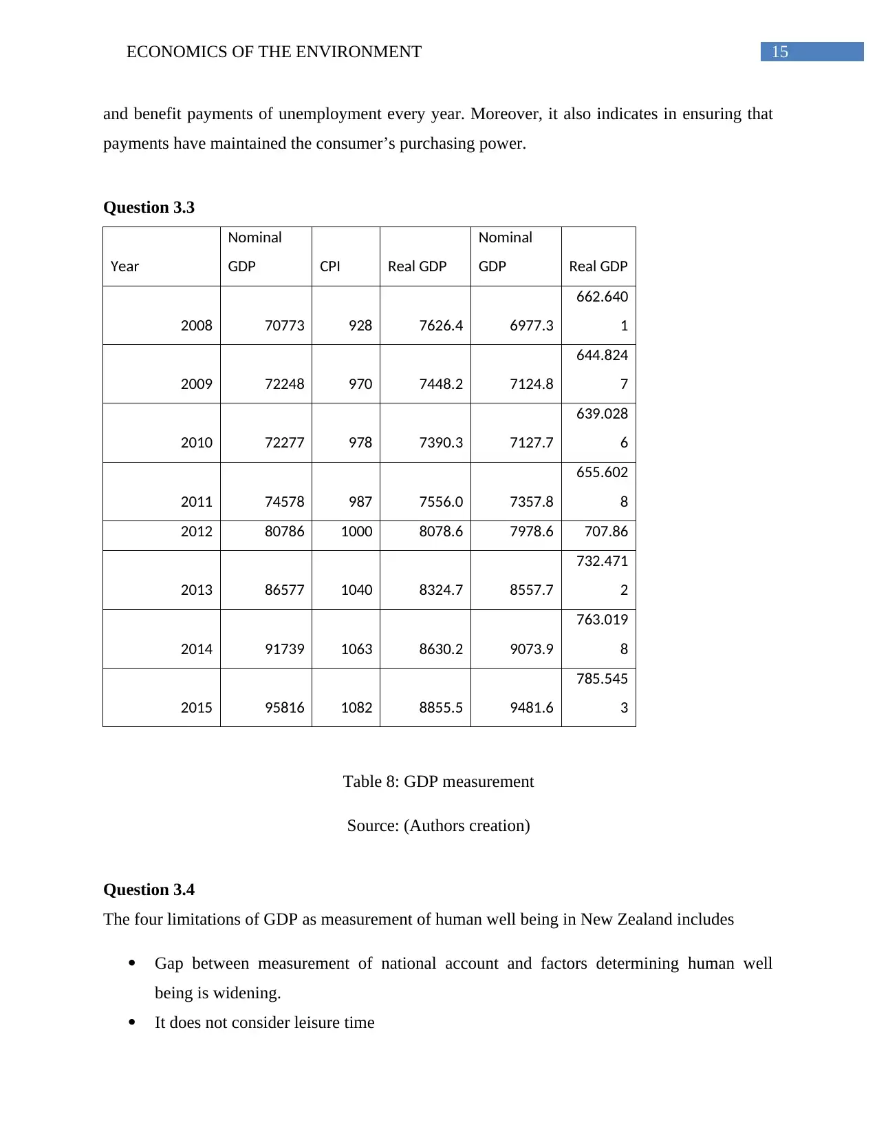
Question 3.3
Year
Nominal
GDP CPI Real GDP
Nominal
GDP Real GDP
2008 70773 928 7626.4 6977.3
662.640
1
2009 72248 970 7448.2 7124.8
644.824
7
2010 72277 978 7390.3 7127.7
639.028
6
2011 74578 987 7556.0 7357.8
655.602
8
2012 80786 1000 8078.6 7978.6 707.86
2013 86577 1040 8324.7 8557.7
732.471
2
2014 91739 1063 8630.2 9073.9
763.019
8
2015 95816 1082 8855.5 9481.6
785.545
3
Table 8: GDP measurement
Source: (Authors creation)
Question 3.4
The four limitations of GDP as measurement of human well being in New Zealand includes
Gap between measurement of national account and factors determining human well
being is widening.
It does not consider leisure time
and benefit payments of unemployment every year. Moreover, it also indicates in ensuring that
payments have maintained the consumer’s purchasing power.
Question 3.3
Year
Nominal
GDP CPI Real GDP
Nominal
GDP Real GDP
2008 70773 928 7626.4 6977.3
662.640
1
2009 72248 970 7448.2 7124.8
644.824
7
2010 72277 978 7390.3 7127.7
639.028
6
2011 74578 987 7556.0 7357.8
655.602
8
2012 80786 1000 8078.6 7978.6 707.86
2013 86577 1040 8324.7 8557.7
732.471
2
2014 91739 1063 8630.2 9073.9
763.019
8
2015 95816 1082 8855.5 9481.6
785.545
3
Table 8: GDP measurement
Source: (Authors creation)
Question 3.4
The four limitations of GDP as measurement of human well being in New Zealand includes
Gap between measurement of national account and factors determining human well
being is widening.
It does not consider leisure time
Secure Best Marks with AI Grader
Need help grading? Try our AI Grader for instant feedback on your assignments.
16ECONOMICS OF THE ENVIRONMENT
The GDP value understates real income changes
It also does not consider the amount of hard work that workers give in producing output.
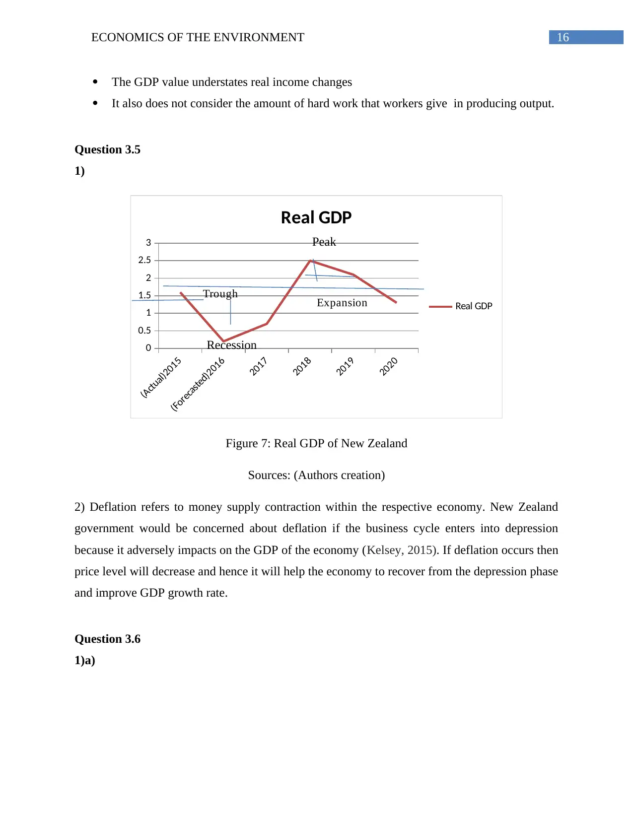
Question 3.5
1)
(Actual)2015
(Forecasted)2016
2017
2018
2019
2020
0
0.5
1
1.5
2
2.5
3
Real GDP
Real GDPExpansion
Trough
Figure 7: Real GDP of New Zealand
Sources: (Authors creation)
2) Deflation refers to money supply contraction within the respective economy. New Zealand
government would be concerned about deflation if the business cycle enters into depression
because it adversely impacts on the GDP of the economy (Kelsey, 2015). If deflation occurs then
price level will decrease and hence it will help the economy to recover from the depression phase
and improve GDP growth rate.
Question 3.6
1)a)
Peak
Recession
The GDP value understates real income changes
It also does not consider the amount of hard work that workers give in producing output.
Question 3.5
1)
(Actual)2015
(Forecasted)2016
2017
2018
2019
2020
0
0.5
1
1.5
2
2.5
3
Real GDP
Real GDPExpansion
Trough
Figure 7: Real GDP of New Zealand
Sources: (Authors creation)
2) Deflation refers to money supply contraction within the respective economy. New Zealand
government would be concerned about deflation if the business cycle enters into depression
because it adversely impacts on the GDP of the economy (Kelsey, 2015). If deflation occurs then
price level will decrease and hence it will help the economy to recover from the depression phase
and improve GDP growth rate.
Question 3.6
1)a)
Peak
Recession
17ECONOMICS OF THE ENVIRONMENT
AD1
AS
P1
Real GDP
Prices
P2
R1 R2
AD2
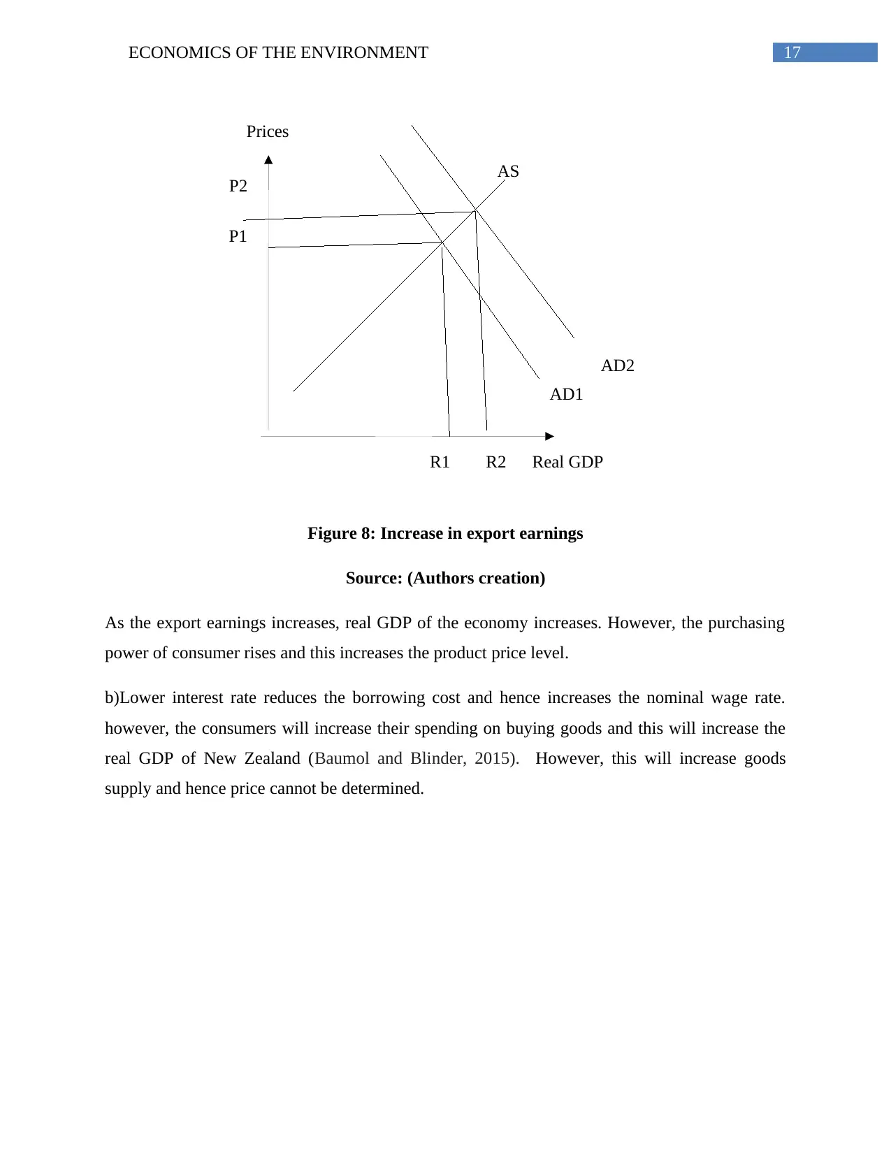
Figure 8: Increase in export earnings
Source: (Authors creation)
As the export earnings increases, real GDP of the economy increases. However, the purchasing
power of consumer rises and this increases the product price level.
b)Lower interest rate reduces the borrowing cost and hence increases the nominal wage rate.
however, the consumers will increase their spending on buying goods and this will increase the
real GDP of New Zealand (Baumol and Blinder, 2015). However, this will increase goods
supply and hence price cannot be determined.
AD1
AS
P1
Real GDP
Prices
P2
R1 R2
AD2
Figure 8: Increase in export earnings
Source: (Authors creation)
As the export earnings increases, real GDP of the economy increases. However, the purchasing
power of consumer rises and this increases the product price level.
b)Lower interest rate reduces the borrowing cost and hence increases the nominal wage rate.
however, the consumers will increase their spending on buying goods and this will increase the
real GDP of New Zealand (Baumol and Blinder, 2015). However, this will increase goods
supply and hence price cannot be determined.
18ECONOMICS OF THE ENVIRONMENT
AS
AD1
AD
AS1
P
R R1 Real GDP
Prices
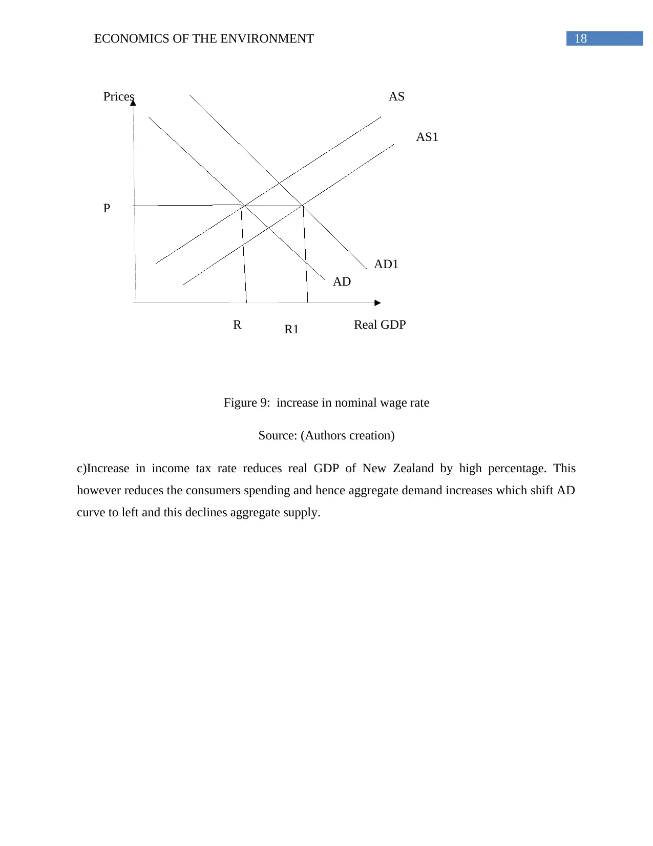
Figure 9: increase in nominal wage rate
Source: (Authors creation)
c)Increase in income tax rate reduces real GDP of New Zealand by high percentage. This
however reduces the consumers spending and hence aggregate demand increases which shift AD
curve to left and this declines aggregate supply.
AS
AD1
AD
AS1
P
R R1 Real GDP
Prices
Figure 9: increase in nominal wage rate
Source: (Authors creation)
c)Increase in income tax rate reduces real GDP of New Zealand by high percentage. This
however reduces the consumers spending and hence aggregate demand increases which shift AD
curve to left and this declines aggregate supply.
Paraphrase This Document
Need a fresh take? Get an instant paraphrase of this document with our AI Paraphraser
19ECONOMICS OF THE ENVIRONMENT
AD
AD1
AS
AS1
P
RR1
P1
Real GDP
Price
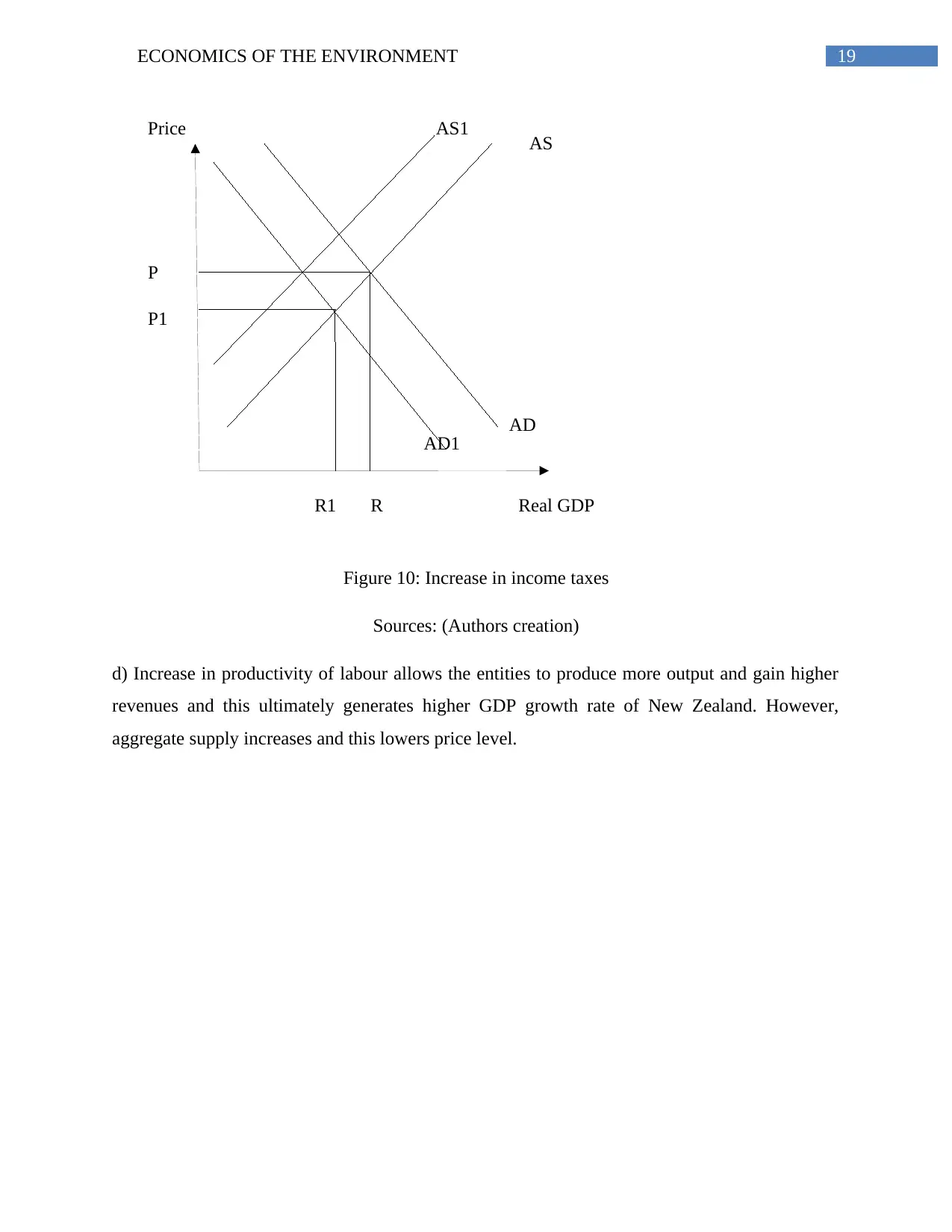
Figure 10: Increase in income taxes
Sources: (Authors creation)
d) Increase in productivity of labour allows the entities to produce more output and gain higher
revenues and this ultimately generates higher GDP growth rate of New Zealand. However,
aggregate supply increases and this lowers price level.
AD
AD1
AS
AS1
P
RR1
P1
Real GDP
Price
Figure 10: Increase in income taxes
Sources: (Authors creation)
d) Increase in productivity of labour allows the entities to produce more output and gain higher
revenues and this ultimately generates higher GDP growth rate of New Zealand. However,
aggregate supply increases and this lowers price level.
20ECONOMICS OF THE ENVIRONMENT
Price
Real GDP
AS
AS1
AD
P
P1
R R1
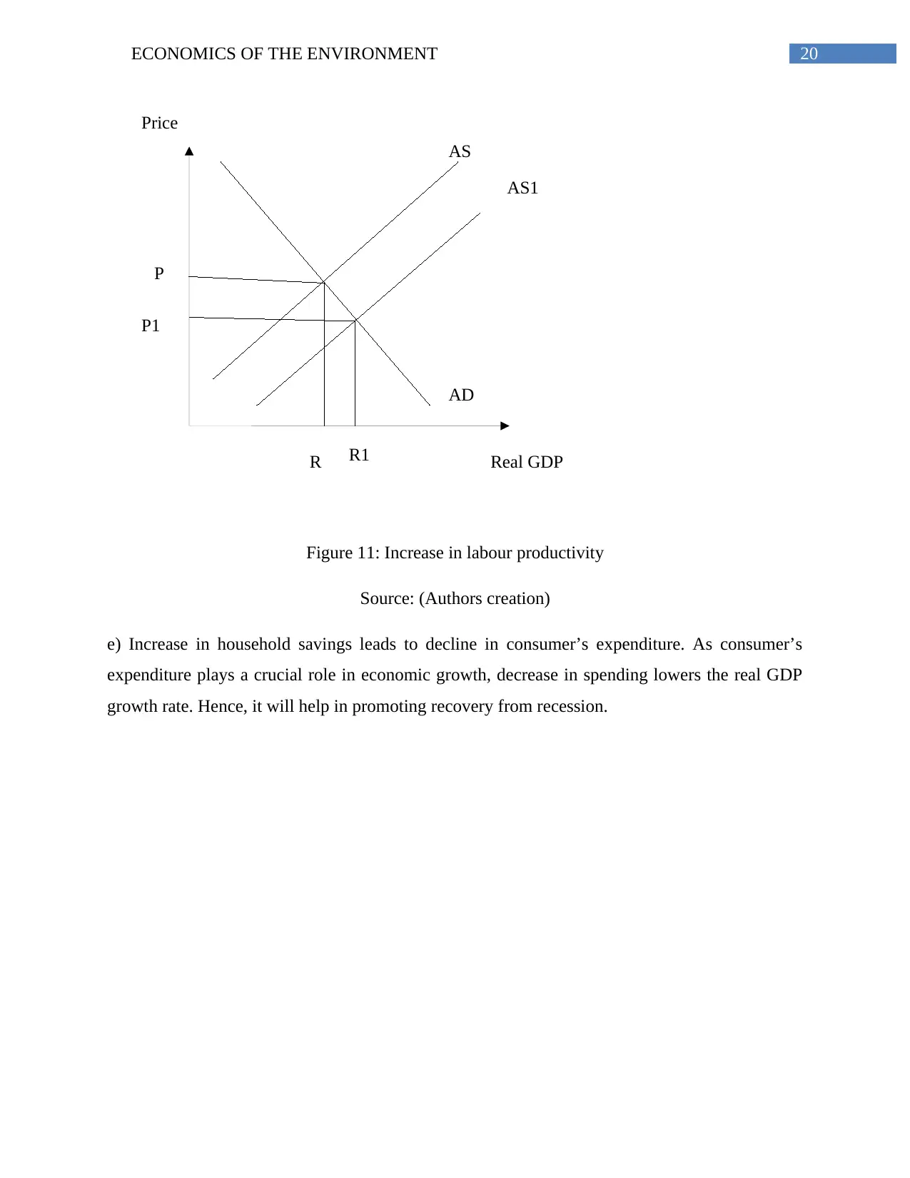
Figure 11: Increase in labour productivity
Source: (Authors creation)
e) Increase in household savings leads to decline in consumer’s expenditure. As consumer’s
expenditure plays a crucial role in economic growth, decrease in spending lowers the real GDP
growth rate. Hence, it will help in promoting recovery from recession.
Price
Real GDP
AS
AS1
AD
P
P1
R R1
Figure 11: Increase in labour productivity
Source: (Authors creation)
e) Increase in household savings leads to decline in consumer’s expenditure. As consumer’s
expenditure plays a crucial role in economic growth, decrease in spending lowers the real GDP
growth rate. Hence, it will help in promoting recovery from recession.
21ECONOMICS OF THE ENVIRONMENT
Real GDP
Price
AS
AD
AD1
P
R1 R
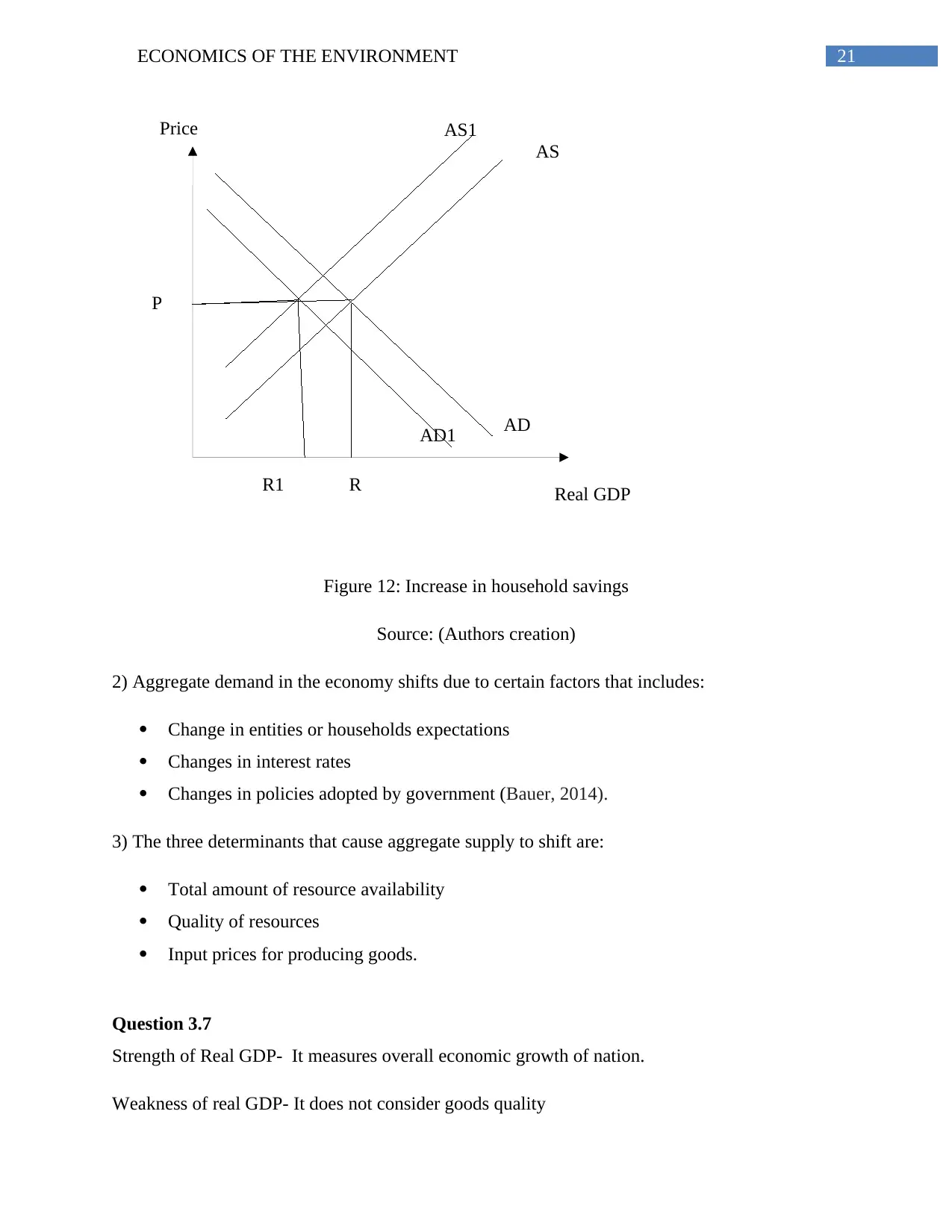
Figure 12: Increase in household savings
Source: (Authors creation)
2) Aggregate demand in the economy shifts due to certain factors that includes:
Change in entities or households expectations
Changes in interest rates
Changes in policies adopted by government (Bauer, 2014).
3) The three determinants that cause aggregate supply to shift are:
Total amount of resource availability
Quality of resources
Input prices for producing goods.
Question 3.7
Strength of Real GDP- It measures overall economic growth of nation.
Weakness of real GDP- It does not consider goods quality
AS1
Real GDP
Price
AS
AD
AD1
P
R1 R
Figure 12: Increase in household savings
Source: (Authors creation)
2) Aggregate demand in the economy shifts due to certain factors that includes:
Change in entities or households expectations
Changes in interest rates
Changes in policies adopted by government (Bauer, 2014).
3) The three determinants that cause aggregate supply to shift are:
Total amount of resource availability
Quality of resources
Input prices for producing goods.
Question 3.7
Strength of Real GDP- It measures overall economic growth of nation.
Weakness of real GDP- It does not consider goods quality
AS1
Secure Best Marks with AI Grader
Need help grading? Try our AI Grader for instant feedback on your assignments.
22ECONOMICS OF THE ENVIRONMENT
Strength of productive capacity- it helps in predicting behavior of business cycle
Weakness of productive capacity- advancement of technology might not have high productive
capacity
Strength of net social welfare- it helps to promote healthy environment in the economy
Weakness of net social welfare- it includes fraud risk within the nation.
23ECONOMICS OF THE ENVIRONMENT
References
Bauer, M. J. R. (2014). Principles of microeconomics.
Baumol, W. J., & Blinder, A. S. (2015). Microeconomics: Principles and policy. Cengage
Learning.
Caragata, P. J. (2012). The economic and compliance consequences of taxation: A report on the
health of the tax system in New Zealand. Springer Science & Business Media.
Fry, J. (2014). Migration and macroeconomic performance in New Zealand: theory and
evidence. The Treasury.
Hall, R. E., & Lieberman, M. (2012). Microeconomics: Principles and applications. Cengage
Learning.
Kelsey, J. (2015). Reclaiming the future: New Zealand and the global economy. Bridget
Williams Books.
Mankiw, N. G. (2014). Principles of macroeconomics. Cengage Learning.
McDowell, R. W., & Nash, D. (2012). A review of the cost-effectiveness and suitability of
mitigation strategies to prevent phosphorus loss from dairy farms in New Zealand and
Australia. Journal of Environmental Quality, 41(3), 680-693.
Rios, M. C., McConnell, C. R., & Brue, S. L. (2013). Economics: Principles, problems, and
policies. McGraw-Hill.
Sikdar, S. (2012). Principles of macroeconomics. OUP Catalogue.
Tinkler, S., & Woods, J. (2013). The readability of principles of macroeconomics textbooks. The
Journal of Economic Education, 44(2), 178-191.
1 out of 24
Related Documents


Your All-in-One AI-Powered Toolkit for Academic Success.
+13062052269
info@desklib.com
Available 24*7 on WhatsApp / Email
![[object Object]](/_next/static/media/star-bottom.7253800d.svg)
Unlock your academic potential
© 2024 | Zucol Services PVT LTD | All rights reserved.