Assignment Sample Solutions and Codes
Added on 2022-09-01
16 Pages6050 Words19 Views
Assighment
Sample Solutions and Codes
3/26/2020
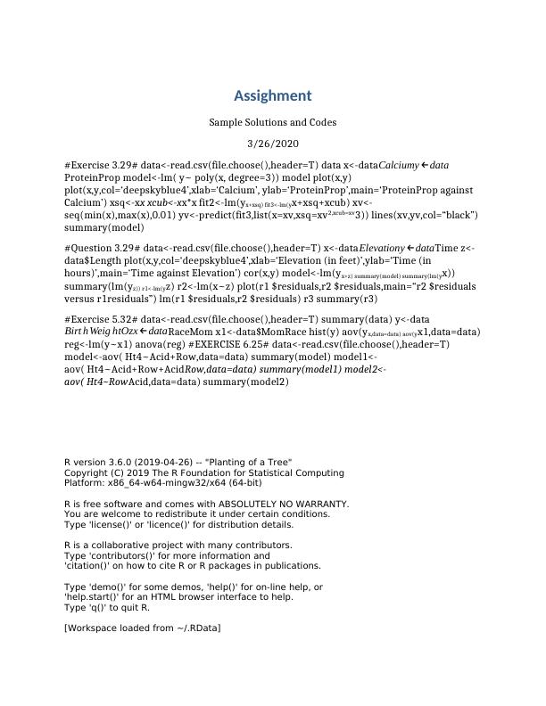
#Exercise 3.29# data<-read.csv(file.choose(),header=T) data x<-data Calciumy ←data
ProteinProp model<-lm( y~ poly(x, degree=3)) model plot(x,y)
plot(x,y,col=‘deepskyblue4’,xlab=‘Calcium’, ylab=‘ProteinProp’,main=‘ProteinProp against
Calcium’) xsq<-xx xcub<-xx*x fit2<-lm(yx+xsq) fit3<-lm(yx+xsq+xcub) xv<-
seq(min(x),max(x),0.01) yv<-predict(fit3,list(x=xv,xsq=xv2,xcub=xv3)) lines(xv,yv,col=“black”)
summary(model)
#Question 3.29# data<-read.csv(file.choose(),header=T) x<-dataElevationy ←dataTime z<-
data$Length plot(x,y,col=‘deepskyblue4’,xlab=‘Elevation (in feet)’,ylab=‘Time (in
hours)’,main=‘Time against Elevation’) cor(x,y) model<-lm(yx+z) summary(model) summary(lm(yx))
summary(lm(yz)) r1<-lm(yz) r2<-lm(x~z) plot(r1 $residuals,r2 $residuals,main=“r2 $residuals
versus r1residuals”) lm(r1 $residuals,r2 $residuals) r3 summary(r3)
#Exercise 5.32# data<-read.csv(file.choose(),header=T) summary(data) y<-data
Birt h Weig htOzx ←dataRaceMom x1<-data$MomRace hist(y) aov(yx,data=data) aov(yx1,data=data)
reg<-lm(y~x1) anova(reg) #EXERCISE 6.25# data<-read.csv(file.choose(),header=T)
model<-aov( Ht4~Acid+Row,data=data) summary(model) model1<-
aov( Ht4~Acid+Row+AcidRow,data=data) summary(model1) model2<-
aov( Ht4~RowAcid,data=data) summary(model2)
R version 3.6.0 (2019-04-26) -- "Planting of a Tree"
Copyright (C) 2019 The R Foundation for Statistical Computing
Platform: x86_64-w64-mingw32/x64 (64-bit)
R is free software and comes with ABSOLUTELY NO WARRANTY.
You are welcome to redistribute it under certain conditions.
Type 'license()' or 'licence()' for distribution details.
R is a collaborative project with many contributors.
Type 'contributors()' for more information and
'citation()' on how to cite R or R packages in publications.
Type 'demo()' for some demos, 'help()' for on-line help, or
'help.start()' for an HTML browser interface to help.
Type 'q()' to quit R.
[Workspace loaded from ~/.RData]
Sample Solutions and Codes
3/26/2020
#Exercise 3.29# data<-read.csv(file.choose(),header=T) data x<-data Calciumy ←data
ProteinProp model<-lm( y~ poly(x, degree=3)) model plot(x,y)
plot(x,y,col=‘deepskyblue4’,xlab=‘Calcium’, ylab=‘ProteinProp’,main=‘ProteinProp against
Calcium’) xsq<-xx xcub<-xx*x fit2<-lm(yx+xsq) fit3<-lm(yx+xsq+xcub) xv<-
seq(min(x),max(x),0.01) yv<-predict(fit3,list(x=xv,xsq=xv2,xcub=xv3)) lines(xv,yv,col=“black”)
summary(model)
#Question 3.29# data<-read.csv(file.choose(),header=T) x<-dataElevationy ←dataTime z<-
data$Length plot(x,y,col=‘deepskyblue4’,xlab=‘Elevation (in feet)’,ylab=‘Time (in
hours)’,main=‘Time against Elevation’) cor(x,y) model<-lm(yx+z) summary(model) summary(lm(yx))
summary(lm(yz)) r1<-lm(yz) r2<-lm(x~z) plot(r1 $residuals,r2 $residuals,main=“r2 $residuals
versus r1residuals”) lm(r1 $residuals,r2 $residuals) r3 summary(r3)
#Exercise 5.32# data<-read.csv(file.choose(),header=T) summary(data) y<-data
Birt h Weig htOzx ←dataRaceMom x1<-data$MomRace hist(y) aov(yx,data=data) aov(yx1,data=data)
reg<-lm(y~x1) anova(reg) #EXERCISE 6.25# data<-read.csv(file.choose(),header=T)
model<-aov( Ht4~Acid+Row,data=data) summary(model) model1<-
aov( Ht4~Acid+Row+AcidRow,data=data) summary(model1) model2<-
aov( Ht4~RowAcid,data=data) summary(model2)
R version 3.6.0 (2019-04-26) -- "Planting of a Tree"
Copyright (C) 2019 The R Foundation for Statistical Computing
Platform: x86_64-w64-mingw32/x64 (64-bit)
R is free software and comes with ABSOLUTELY NO WARRANTY.
You are welcome to redistribute it under certain conditions.
Type 'license()' or 'licence()' for distribution details.
R is a collaborative project with many contributors.
Type 'contributors()' for more information and
'citation()' on how to cite R or R packages in publications.
Type 'demo()' for some demos, 'help()' for on-line help, or
'help.start()' for an HTML browser interface to help.
Type 'q()' to quit R.
[Workspace loaded from ~/.RData]
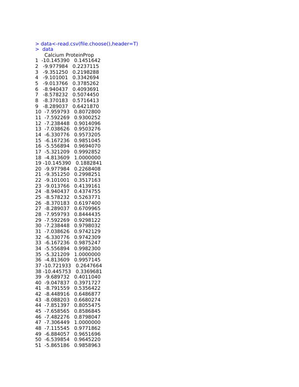
> data<-read.csv(file.choose(),header=T)
> data
Calcium ProteinProp
1 -10.145390 0.1451642
2 -9.977984 0.2237115
3 -9.351250 0.2198288
4 -9.101001 0.3342694
5 -9.013766 0.3785262
6 -8.940437 0.4093691
7 -8.578232 0.5074450
8 -8.370183 0.5716413
9 -8.289037 0.6421870
10 -7.959793 0.8072800
11 -7.592269 0.9300252
12 -7.238448 0.9014096
13 -7.038626 0.9503276
14 -6.330776 0.9573205
15 -6.167236 0.9851045
16 -5.556894 0.9694070
17 -5.321209 0.9992852
18 -4.813609 1.0000000
19 -10.145390 0.1882841
20 -9.977984 0.2268408
21 -9.351250 0.2998251
22 -9.101001 0.3517163
23 -9.013766 0.4139161
24 -8.940437 0.4374755
25 -8.578232 0.5263771
26 -8.370183 0.6197400
27 -8.289037 0.6709965
28 -7.959793 0.8444435
29 -7.592269 0.9298122
30 -7.238448 0.9798032
31 -7.038626 0.9742129
32 -6.330776 0.9742309
33 -6.167236 0.9875247
34 -5.556894 0.9982300
35 -5.321209 1.0000000
36 -4.813609 0.9957145
37 -10.721933 0.2647664
38 -10.445753 0.3369681
39 -9.689732 0.4011040
40 -9.047837 0.3971727
41 -8.791559 0.5356422
42 -8.448916 0.6486877
43 -8.088203 0.6680274
44 -7.851397 0.8055475
45 -7.658565 0.8586845
46 -7.482276 0.8798047
47 -7.306449 1.0000000
48 -7.115545 0.9771862
49 -6.884057 0.9651696
50 -6.539854 0.9645220
51 -5.865186 0.9858963
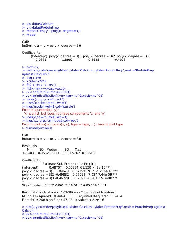
> x<-data$Calcium
> y<-data$ProteinProp
> model<-lm( y~ poly(x, degree=3))
> model
Call:
lm(formula = y ~ poly(x, degree = 3))
Coefficients:
(Intercept) poly(x, degree = 3)1 poly(x, degree = 3)2 poly(x, degree = 3)3
0.6871 1.8962 -0.4988 -0.4673
> plot(x,y)
> plot(x,y,col='deepskyblue4',xlab='Calcium', ylab='ProteinProp',main='ProteinProp
against Calcium ')
> xsq<-x*x
> xcub<-x*x*x
> fit2<-lm(y~x+xsq)
> fit3<-lm(y~x+xsq+xcub)
> xv<-seq(min(x),max(x),0.01)
> yv<-predict(fit3,list(x=xv,xsq=xv^2,xcub=xv^3))
> lines(xv,yv,col="black")
> lines(x,col='green',lwd=3)
> lines(model,lwd=3,col='purple')
Error in xy.coords(x, y) :
'x' is a list, but does not have components 'x' and 'y'
> lines(y,col='purple',lwd=3)
> lines(x,y,predict(model),col='red')
Error in plot.xy(xy.coords(x, y), type = type, ...) : invalid plot type
> summary(model)
Call:
lm(formula = y ~ poly(x, degree = 3))
Residuals:
Min 1Q Median 3Q Max
-0.14031 -0.05528 -0.01859 0.05267 0.13583
Coefficients:
Estimate Std. Error t value Pr(>|t|)
(Intercept) 0.68707 0.00994 69.120 < 2e-16 ***
poly(x, degree = 3)1 1.89623 0.07099 26.712 < 2e-16 ***
poly(x, degree = 3)2 -0.49882 0.07099 -7.027 7.44e-09 ***
poly(x, degree = 3)3 -0.46729 0.07099 -6.583 3.51e-08 ***
---
Signif. codes: 0 ‘***’ 0.001 ‘**’ 0.01 ‘*’ 0.05 ‘.’ 0.1 ‘ ’ 1
Residual standard error: 0.07099 on 47 degrees of freedom
Multiple R-squared: 0.9449, Adjusted R-squared: 0.9414
F-statistic: 268.8 on 3 and 47 DF, p-value: < 2.2e-16
> plot(x,y,col='deepskyblue4',xlab='Calcium', ylab='ProteinProp',main='ProteinProp against
Calcium ')
> xv<-seq(min(x),max(x),0.01)
> yv<-predict(fit3,list(x=xv,xsq=xv^2,xcub=xv^3))
> lines(xv,yv,col="black")
> data<-read.csv(file.choose(),header=T)
> r1<-lm(y~z)
Error in eval(predvars, data, env) : object 'z' not found
> r2<-lm(x~z)
Error in eval(predvars, data, env) : object 'z' not found
> plot(r1$residuals,r2$residuals)
Error in plot(r1$residuals, r2$residuals) : object 'r1' not found
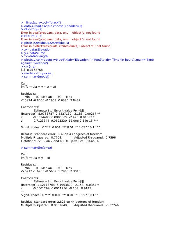
> x<-data$Elevation
> y<-data$Time
> z<-data$Length
> plot(x,y,col='deepskyblue4',xlab='Elevation (in feet)',ylab='Time (in hours)',main='Time
against Elevation')
> cor(x,y)
[1] -0.0162768
> model<-lm(y~x+z)
> summary(model)
Call:
lm(formula = y ~ x + z)
Residuals:
Min 1Q Median 3Q Max
-2.5924 -0.8050 -0.1959 0.6380 3.8432
Coefficients:
Estimate Std. Error t value Pr(>|t|)
(Intercept) 8.0753787 2.5327132 3.188 0.00267 **
x -0.0014483 0.0005805 -2.495 0.01653 *
z 0.7123344 0.0593330 12.006 2.54e-15 ***
---
Signif. codes: 0 ‘***’ 0.001 ‘**’ 0.01 ‘*’ 0.05 ‘.’ 0.1 ‘ ’ 1
Residual standard error: 1.37 on 43 degrees of freedom
Multiple R-squared: 0.7703, Adjusted R-squared: 0.7596
F-statistic: 72.09 on 2 and 43 DF, p-value: 1.844e-14
> summary(lm(y~x))
Call:
lm(formula = y ~ x)
Residuals:
Min 1Q Median 3Q Max
-5.6912 -1.6985 -0.5639 1.2963 7.3015
Coefficients:
Estimate Std. Error t value Pr(>|t|)
(Intercept) 11.2113764 5.1953800 2.158 0.0364 *
x -0.0001269 0.0011756 -0.108 0.9145
---
Signif. codes: 0 ‘***’ 0.001 ‘**’ 0.01 ‘*’ 0.05 ‘.’ 0.1 ‘ ’ 1
Residual standard error: 2.826 on 44 degrees of freedom
Multiple R-squared: 0.0002649, Adjusted R-squared: -0.02246
> data<-read.csv(file.choose(),header=T)
> r1<-lm(y~z)
Error in eval(predvars, data, env) : object 'z' not found
> r2<-lm(x~z)
Error in eval(predvars, data, env) : object 'z' not found
> plot(r1$residuals,r2$residuals)
Error in plot(r1$residuals, r2$residuals) : object 'r1' not found
> x<-data$Elevation
> y<-data$Time
> z<-data$Length
> plot(x,y,col='deepskyblue4',xlab='Elevation (in feet)',ylab='Time (in hours)',main='Time
against Elevation')
> cor(x,y)
[1] -0.0162768
> model<-lm(y~x+z)
> summary(model)
Call:
lm(formula = y ~ x + z)
Residuals:
Min 1Q Median 3Q Max
-2.5924 -0.8050 -0.1959 0.6380 3.8432
Coefficients:
Estimate Std. Error t value Pr(>|t|)
(Intercept) 8.0753787 2.5327132 3.188 0.00267 **
x -0.0014483 0.0005805 -2.495 0.01653 *
z 0.7123344 0.0593330 12.006 2.54e-15 ***
---
Signif. codes: 0 ‘***’ 0.001 ‘**’ 0.01 ‘*’ 0.05 ‘.’ 0.1 ‘ ’ 1
Residual standard error: 1.37 on 43 degrees of freedom
Multiple R-squared: 0.7703, Adjusted R-squared: 0.7596
F-statistic: 72.09 on 2 and 43 DF, p-value: 1.844e-14
> summary(lm(y~x))
Call:
lm(formula = y ~ x)
Residuals:
Min 1Q Median 3Q Max
-5.6912 -1.6985 -0.5639 1.2963 7.3015
Coefficients:
Estimate Std. Error t value Pr(>|t|)
(Intercept) 11.2113764 5.1953800 2.158 0.0364 *
x -0.0001269 0.0011756 -0.108 0.9145
---
Signif. codes: 0 ‘***’ 0.001 ‘**’ 0.01 ‘*’ 0.05 ‘.’ 0.1 ‘ ’ 1
Residual standard error: 2.826 on 44 degrees of freedom
Multiple R-squared: 0.0002649, Adjusted R-squared: -0.02246
End of preview
Want to access all the pages? Upload your documents or become a member.
Related Documents
Loading Required Package Assignmentlg...
|20
|3180
|36
Data Analysis Project for Deskliblg...
|9
|2087
|218
Regression Analysis | Assignment-1lg...
|7
|872
|19