Vibration Analysis and Modeling of Automobile Suspension Systems

This article discusses the modeling and analysis of single, double, and triple degree of freedom automobile suspension systems. It covers the equations of motion, natural frequencies, and damping ratios, as well as MATLAB implementation and Simulink models for system analysis. The article also includes information on vibration test rig control and roller mechanism applications.

DEMONSTRATION QUESTIONS
By (Name)
INSTITUTIONAL AFFILIATION
COURSE NAME & ID
PROFESSOR (INSTRUCTOR)
LOCATION (STATE, COUNTRY)
DATE OF SUBMISSION
1

SECTION A
QUESTION I: 1 DOF MODELLING
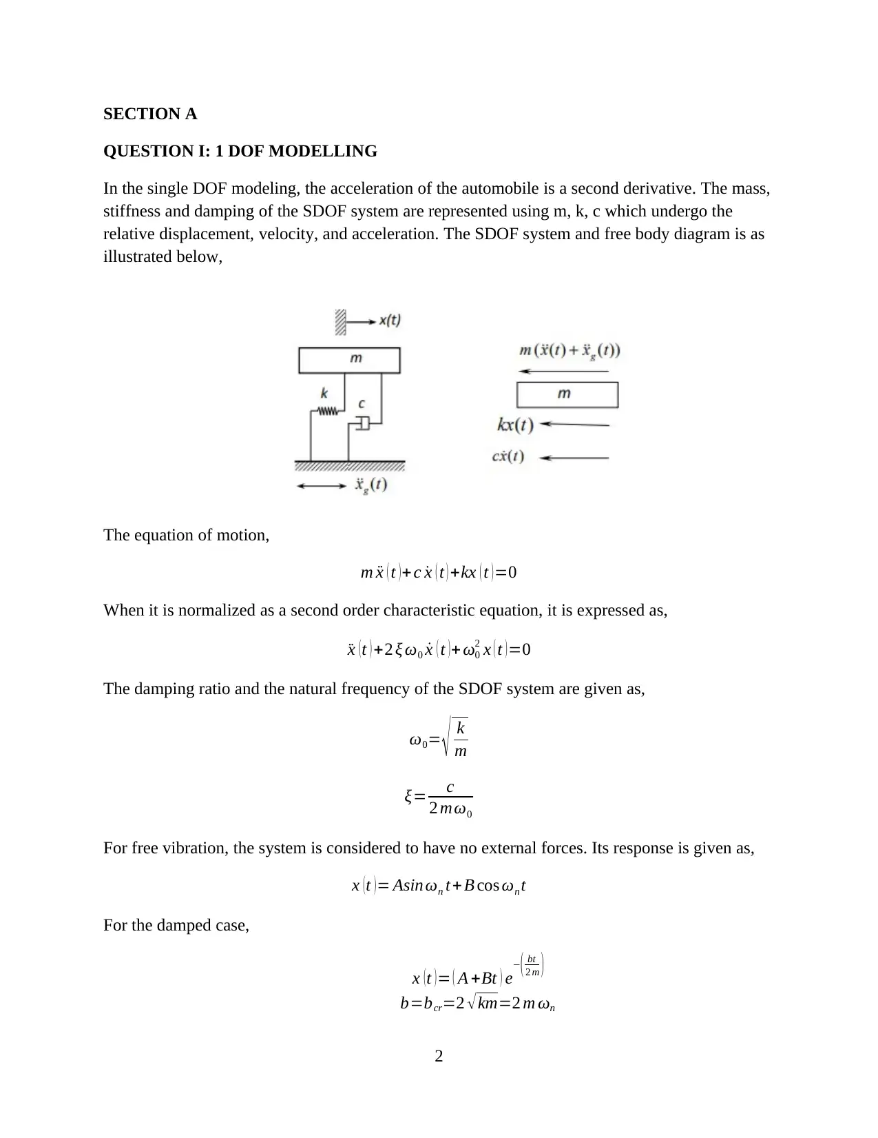
In the single DOF modeling, the acceleration of the automobile is a second derivative. The mass,
stiffness and damping of the SDOF system are represented using m, k, c which undergo the
relative displacement, velocity, and acceleration. The SDOF system and free body diagram is as
illustrated below,
The equation of motion,
m ¨x ( t ) + c ˙x ( t ) +kx ( t ) =0
When it is normalized as a second order characteristic equation, it is expressed as,
¨x (t ) +2 ξ ω0 ˙x ( t )+ ω0
2 x ( t )=0
The damping ratio and the natural frequency of the SDOF system are given as,
ω0= √ k
m
ξ= c
2 mω0
For free vibration, the system is considered to have no external forces. Its response is given as,
x ( t ) = Asin ωn t +B cos ωn t
For the damped case,
x ( t ) = ( A +Bt ) e−( bt
2 m )
b=bcr=2 √km=2 m ωn
2

For the under-damped case,
b< bcr
x (t )=e−( bt
2 m ) ( A sin ωd t + B cos ωd t )
The damping natural frequency of the SDOF system is given as,
ωd=ω0 √ 1−ξ2
For the forced vibration, there is an external force towards the SDOF system, and the general
solution to the characteristic equation is obtained as,
¨x ( t ) + k
m x ( t ) + c
m ˙x ( t ) =Fsin ωt
x (t )= F sin ωt +θ
k
√ (1−
( ω2
ωn
2 ) )+ ( 2 ξω
ωn )2
¿ F
k
( sin ωt +θ
√ ( 1− ( ω2
ωn
2 ) ) +
( 2 ξω
ωn )
2
)
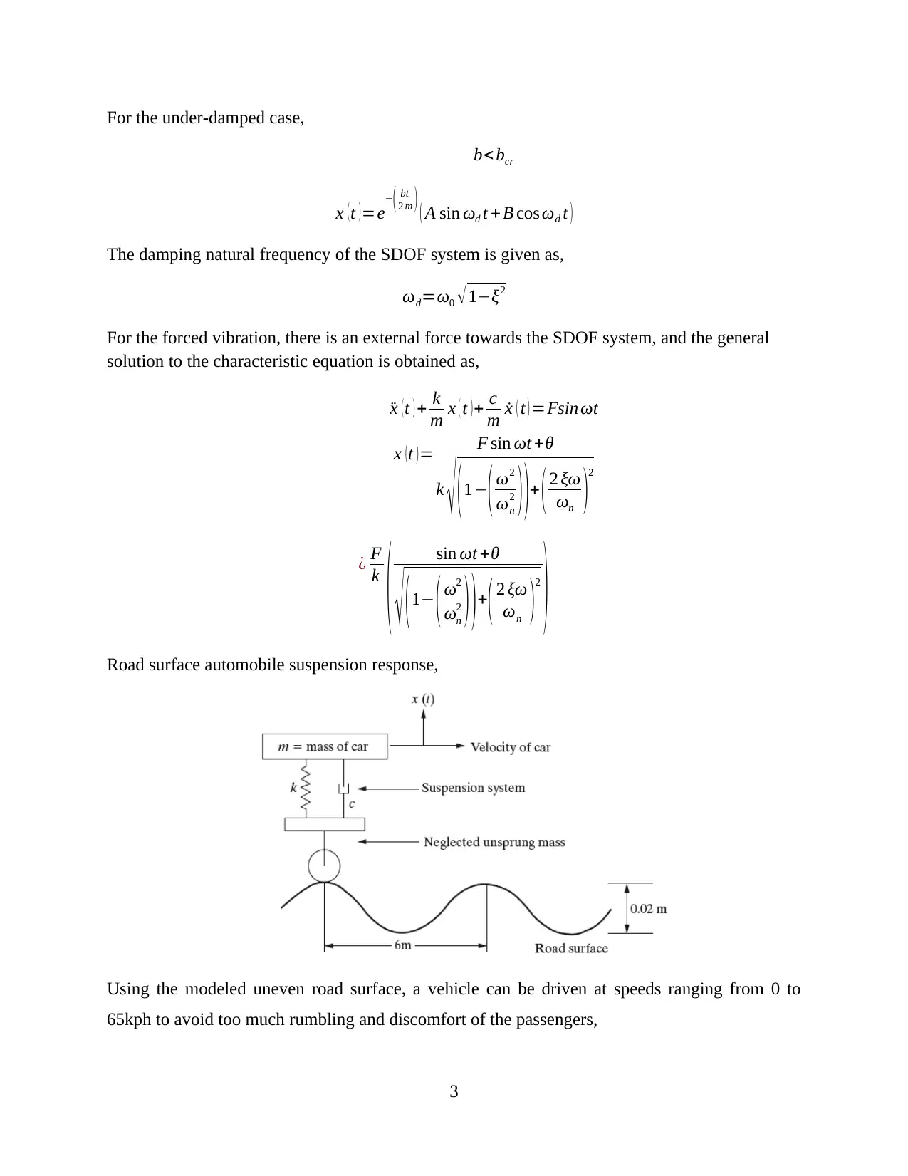
Road surface automobile suspension response,
Using the modeled uneven road surface, a vehicle can be driven at speeds ranging from 0 to
65kph to avoid too much rumbling and discomfort of the passengers,
3

MATLAB implementation of the SDOF System
(i) Obtaining the system Laplace transform and developing a transfer function
(ii) Generating a Simulink model of the system
(iii) Performing several analysis on bode diagrams of the system response, magnification
and transmissibility factor, and derivation of some parameters.
The code snippet
%% SDOF System analysis
m=45e3; % 45000 kg
k=35e3; % stiffness of the spring
c=18500; % damping coefficient, of the damper
% Using matrix form of the SDOF system to generate the
transfer function
A=tf([m c k],[1]) % The transfer function, A
B=tf([c k],[1]) % The transfer function, B
sys=B/A % The transfer function, The system
%% Using the step function to determine the system response
figure(2)
step(sys)
grid on
%% To determine the system magnitude and phase plot using bode
diagram
figure(3)
bode(sys)
grid on
%% The natural frequency and the damping factor of the
calculations in the system
[Wn, zeta]=damp(sys)
4

5

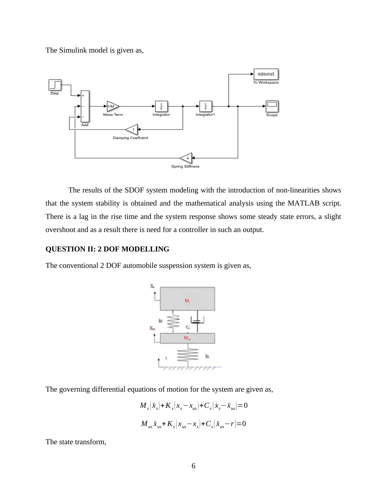
The Simulink model is given as,
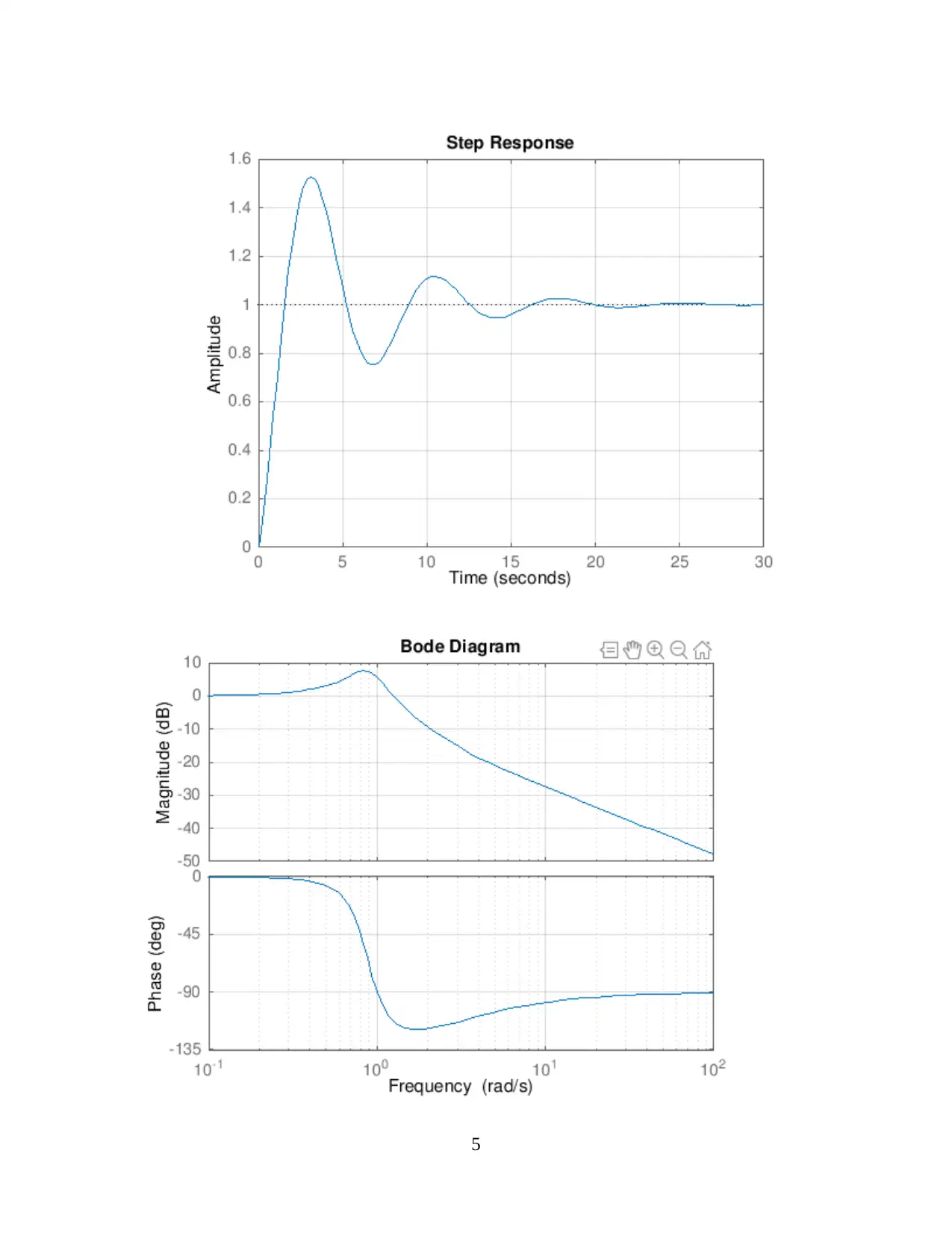
The results of the SDOF system modeling with the introduction of non-linearities shows
that the system stability is obtained and the mathematical analysis using the MATLAB script.
There is a lag in the rise time and the system response shows some steady state errors, a slight
overshoot and as a result there is need for a controller in such an output.
QUESTION II: 2 DOF MODELLING
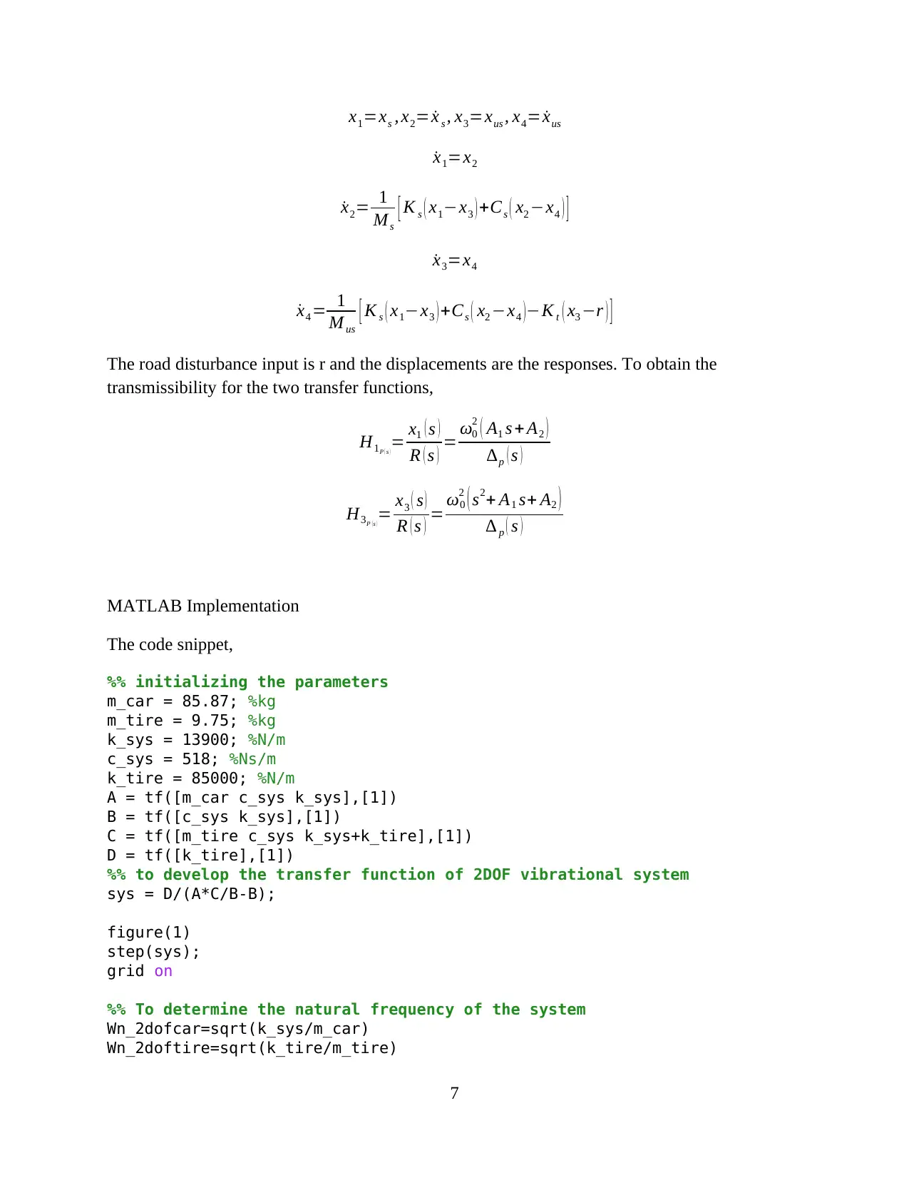
The conventional 2 DOF automobile suspension system is given as,
The governing differential equations of motion for the system are given as,
M s ( ¨xs ) + K s ( xs −xus ) +Cs ( ˙xs− ¨xus ) =0
M us ¨xus+ Ks ( xus−xs ) +Cs ( ¨xus−r )=0
The state transform,
6

x1=xs , x2= ˙x s , x3=xus , x4= ˙xus
˙x1=x2
˙x2= 1
Ms
[ K s ( x1−x3 ) +Cs ( x2 −x4 ) ]
˙x3=x4
˙x4 = 1
M us
[ K s ( x1−x3 ) +Cs ( x2 −x4 )−K t ( x3 −r ) ]
The road disturbance input is r and the displacements are the responses. To obtain the
transmissibility for the two transfer functions,
H1P ( s )
= x1 ( s )
R ( s ) = ω0
2 ( A1 s + A2 )
∆p ( s )
H3P (s )
= x3 ( s )
R ( s ) = ω0
2 ( s2+ A1 s+ A2 )
∆ p ( s )
MATLAB Implementation
The code snippet,
%% initializing the parameters
m_car = 85.87; %kg
m_tire = 9.75; %kg
k_sys = 13900; %N/m
c_sys = 518; %Ns/m
k_tire = 85000; %N/m
A = tf([m_car c_sys k_sys],[1])
B = tf([c_sys k_sys],[1])
C = tf([m_tire c_sys k_sys+k_tire],[1])
D = tf([k_tire],[1])
%% to develop the transfer function of 2DOF vibrational system
sys = D/(A*C/B-B);
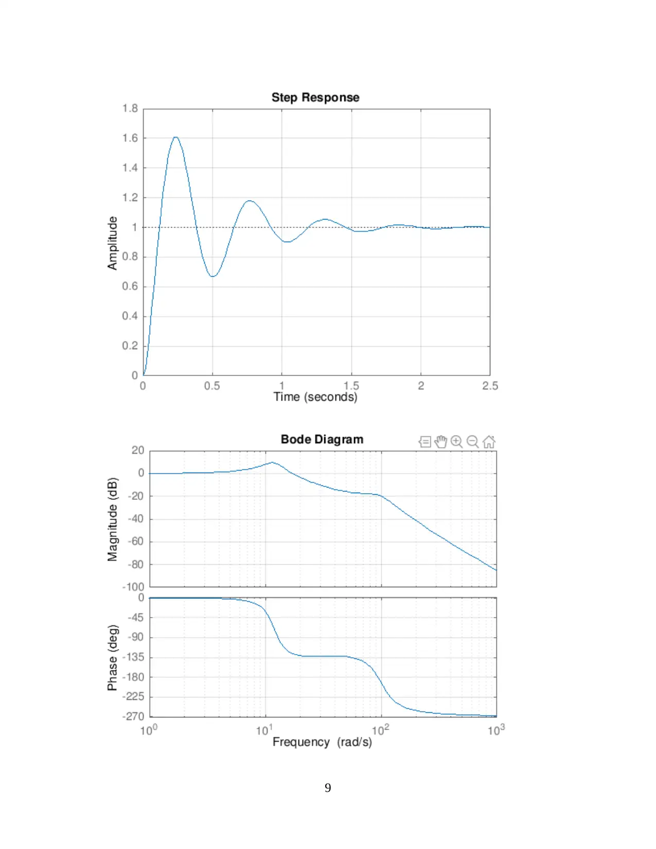
figure(1)
step(sys);
grid on
%% To determine the natural frequency of the system
Wn_2dofcar=sqrt(k_sys/m_car)
Wn_2doftire=sqrt(k_tire/m_tire)
7

%% To determine the mode shapes and natural frequency of the system
... using a plot
figure(2)
bode(sys) %magnitude and phase plots
grid on
%% To obtain the eigenvalues and eigenvectors of the system
r1=k_sys+k_tire-(m_car*Wn_2dofcar^2)
r2=k_tire -(m_tire*Wn_2doftire^2)
r_sys=[r1 -k_tire;-k_tire r2];
eig_val=det(r_sys)
% To determine the system’s eigenvector:
r_sys1=r_sys^-1
b_out=[0;0];
eig_vec=r_sys1*b_out
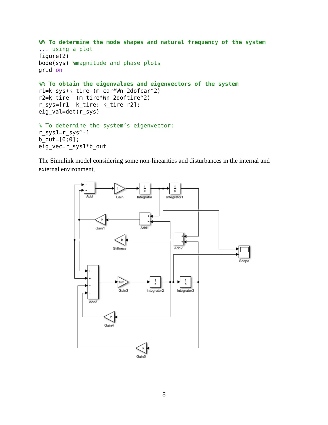
The Simulink model considering some non-linearities and disturbances in the internal and
external environment,
8

9

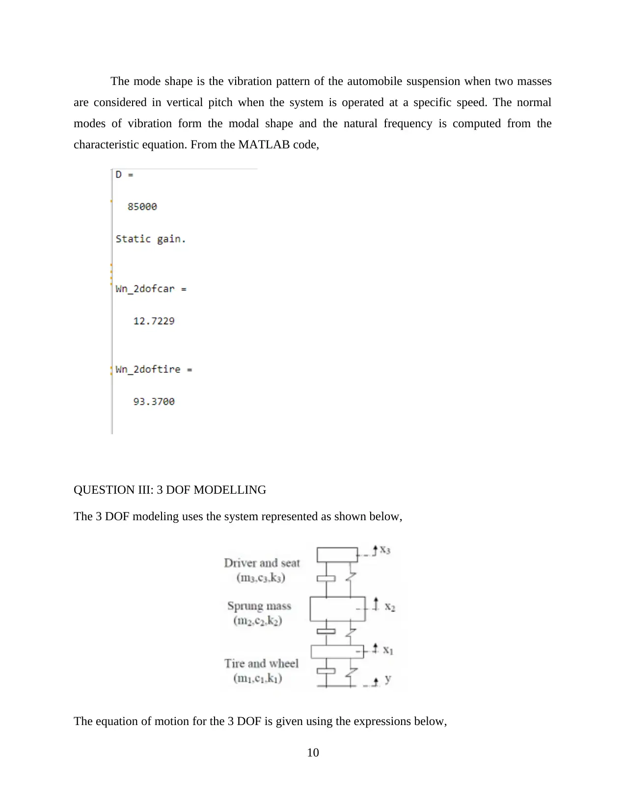
The mode shape is the vibration pattern of the automobile suspension when two masses
are considered in vertical pitch when the system is operated at a specific speed. The normal
modes of vibration form the modal shape and the natural frequency is computed from the
characteristic equation. From the MATLAB code,
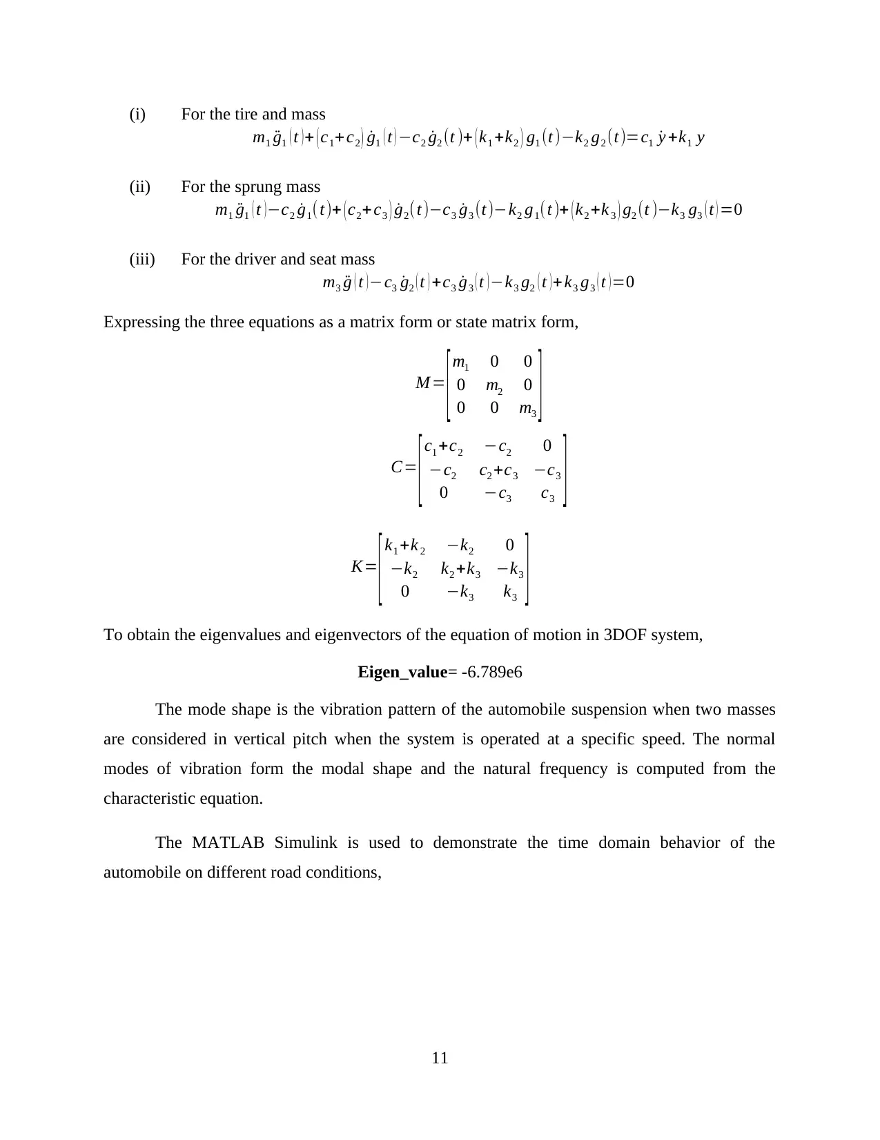
QUESTION III: 3 DOF MODELLING
The 3 DOF modeling uses the system represented as shown below,
The equation of motion for the 3 DOF is given using the expressions below,
10

(i) For the tire and mass
m1 ¨g1 ( t ) + ( c1+c2 ) ˙g1 ( t ) −c2 ˙g2 (t )+ ( k1 +k2 ) g1 (t)−k2 g2 (t)=c1 ˙y +k1 y
(ii) For the sprung mass
m1 ¨g1 ( t ) −c2 ˙g1(t)+ ( c2+c3 ) ˙g2(t)−c3 ˙g3 (t)−k2 g1(t )+ ( k2 +k 3 ) g2 (t )−k3 g3 ( t ) =0
(iii) For the driver and seat mass
m3 ¨g ( t ) −c3 ˙g2 ( t ) +c3 ˙g3 ( t ) −k3 g2 ( t ) + k3 g3 ( t ) =0
Expressing the three equations as a matrix form or state matrix form,
M =
[ m1 0 0
0 m2 0
0 0 m3 ]
C=
[c1 +c2 −c2 0
−c2 c2 +c3 −c3
0 −c3 c3 ]
K=
[ k1 +k 2 −k2 0
−k2 k2 +k3 −k3
0 −k3 k3 ]
To obtain the eigenvalues and eigenvectors of the equation of motion in 3DOF system,
Eigen_value= -6.789e6
The mode shape is the vibration pattern of the automobile suspension when two masses
are considered in vertical pitch when the system is operated at a specific speed. The normal
modes of vibration form the modal shape and the natural frequency is computed from the
characteristic equation.
The MATLAB Simulink is used to demonstrate the time domain behavior of the
automobile on different road conditions,
11

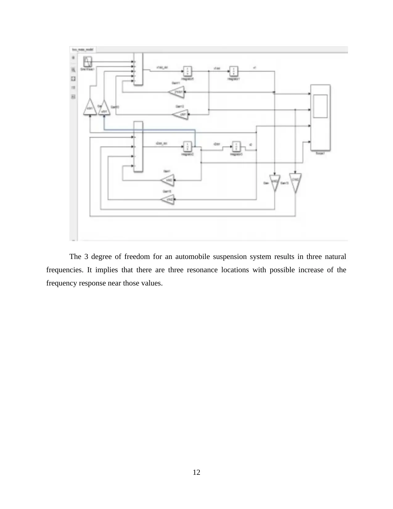
The 3 degree of freedom for an automobile suspension system results in three natural
frequencies. It implies that there are three resonance locations with possible increase of the
frequency response near those values.
12

SECTION B
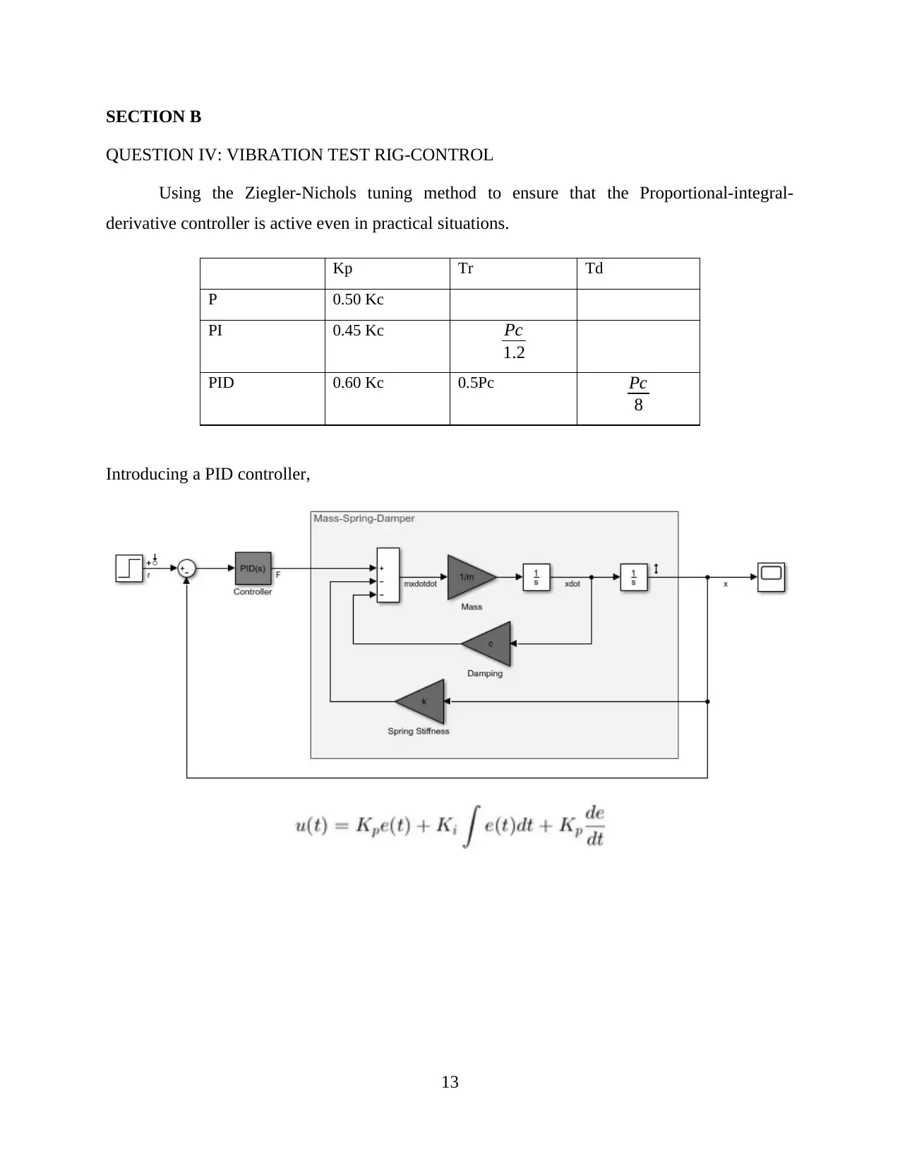
QUESTION IV: VIBRATION TEST RIG-CONTROL
Using the Ziegler-Nichols tuning method to ensure that the Proportional-integral-
derivative controller is active even in practical situations.
Kp Tr Td
P 0.50 Kc
PI 0.45 Kc Pc
1.2
PID 0.60 Kc 0.5Pc Pc
8
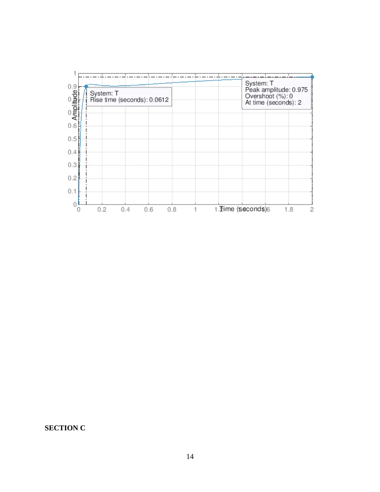
Introducing a PID controller,
13

SECTION C
14

QUESTION V: ROLLER MECHANISM – OTHER VIBRATION APPLICATIONS
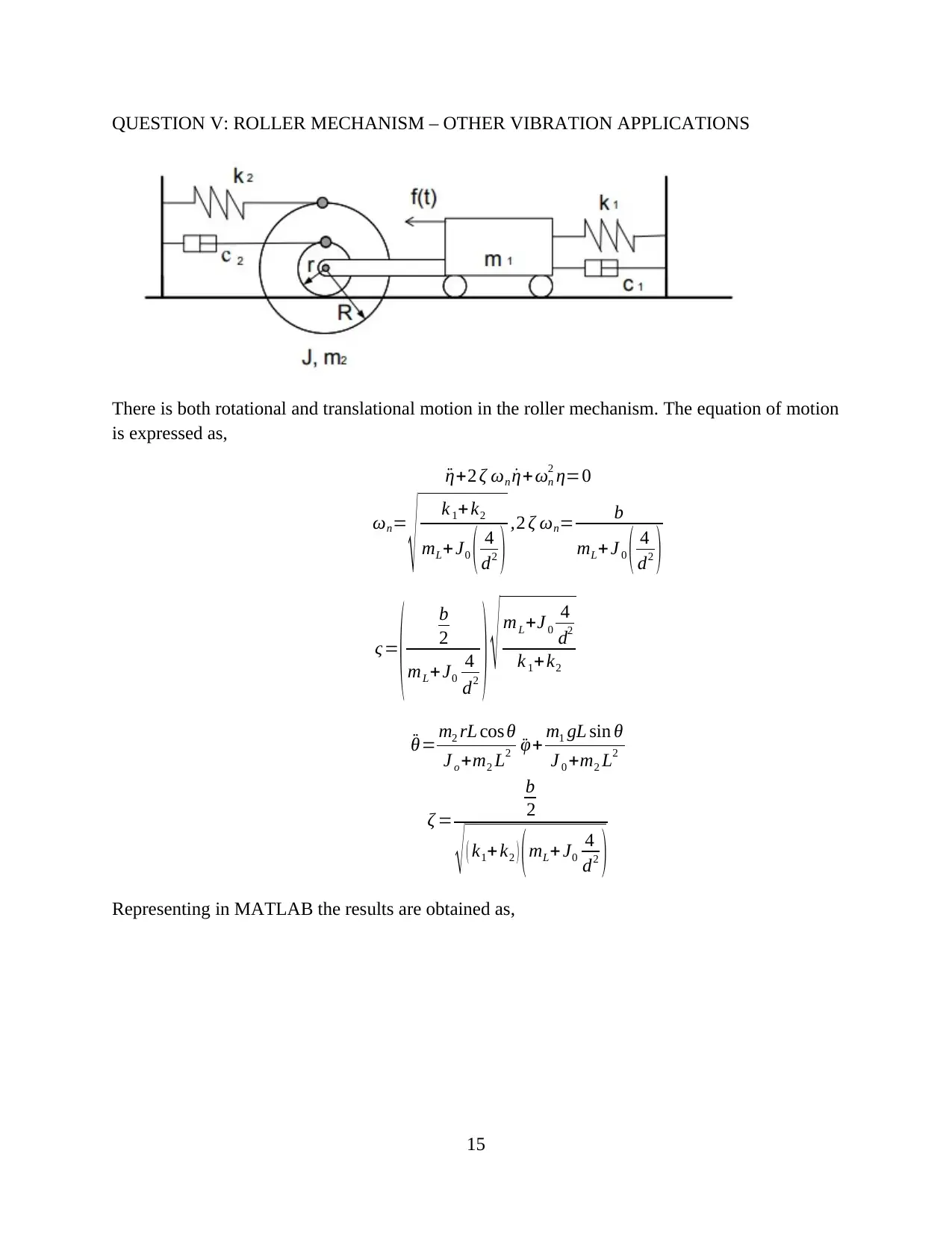
There is both rotational and translational motion in the roller mechanism. The equation of motion
is expressed as,
¨η+2 ζ ωn ˙η+ωn
2 η=0
ωn=
√ k 1+ k2
mL+ J0 ( 4
d2 ) ,2 ζ ωn= b
mL+ J 0 ( 4
d2 )
ς=
( b
2
mL+J0
4
d2 ) √ mL+J 0
4
d2
k 1+k2
¨θ= m2 rL cos θ
J o +m2 L2 ¨φ+ m1 gL sin θ
J 0 +m2 L2
ζ =
b
2
√ ( k1+ k2 ) (mL+ J0
4
d2 )
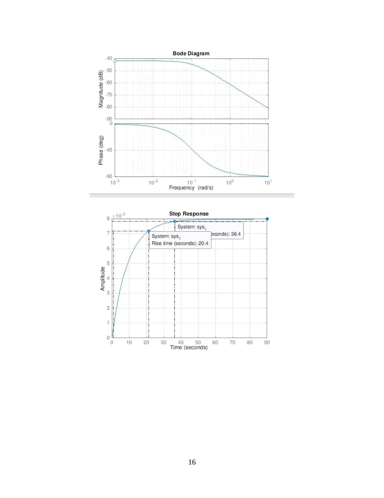
Representing in MATLAB the results are obtained as,
15

16

REFERENCES
Alexandru, C. (2018). Method for the quasi-static analysis of beam axle suspension systems used
for road vehicles. Proceedings of the Institution of Mechanical Engineers, Part D: Journal of
Automobile Engineering, p.095440701879015.
Bankar, A. (2017). Development Using Simulation on a 4-DOF Passive Suspension System with
Thorax-Pelvis. IOSR Journal of Mechanical and Civil Engineering, 17(10), pp.39-45.
He, J. and Fu, Z. (2001). Modal analysis. Oxford [u.a.]: Butterworth-Heinemann.
Iosr-journals.org. (2018). [online] Available at: http://iosrjournals.org/iosr-jmce/papers/RDME-
Volume1/RDME-4.pdf [Accessed 5 Oct. 2018].
Sauder, H. and Sarkar, P. (2017). A 3-DOF forced vibration system for time-domain aeroelastic
parameter identification. Wind and Structures, 24(5), pp.481-500.
Smeringaiova, A., Vojtko, I. and Leskova, B. (2016). Suspension system in automobile system.
Mm Science Journal, 2016(03), pp.1004-1008.
17