Prediction of Financial Distress among Swedish Listed Companies

This thesis examines the prediction of financial distress among Swedish listed companies using Ohlson's O-score and an alteration of the model using Swedish data. It compares the results of three different models derived through logistic regression analysis and finds that a revised model incorporating information related to the audit report and the opinion expressed by the auditor improves the prediction of financial distress. The study aims to provide a model that can be easily understood and applied by investors in Swedish stocks.

Bachelor’s Thesis in Accounting and Financial Management
Stockholm School of Economics
Spring 2012
Prediction of Financial Distress among Swedish Listed Companies
- A study of Ohlson’s O-score and an alteration of the model using Swedish data
Niklas Alyhr* Mattias Holmberg
Instructor: Håkan Thorsell
Date: 30 May 2012
Location: Stockholm School of Economics, Room 538
*[e-mail] [e-mail]

2
ABSTRACT
The prediction of bankruptcy and financial distress related to companies has interested many
researchers and two of the more notable published contributions are attributable to Altman
(1968) and Ohlson (1980). As the studies within this field of research are many, few can be
been related to Swedish listed companies. This thesis mimics the research done by Ohlson in
the pursuit of trying to find a model suitable for the Swedish stock market, with a starting
point in the studies of the same. By comparing the results of three different models derived
through logistic regression analysis, Ohlson’s model still seems to provide some usable input.
However, the results indicate that a revised model, incorporating information related to the
audit report and the opinion expressed by the auditor, improves the prediction of financial
distress among Swedish listed companies. We found this model, Model B, to be the most
suitable one amongst the three.
Key words: Bankruptcy, Financial distress, Prediction model, Audit report, O-score, Swedish
listed companies

3
TABLE OF CONTENTS
Abstract ...................................................................................................................................... 2
1 Introduction ............................................................................................................................. 5
1.1 Purpose ................................................................................................................................. 7
1.2 Question Formulations ......................................................................................................... 7
2 Literature Review .................................................................................................................... 9
2.1 Early Seminal Research: Beaver and Altman................................................................... 9
2.2 Logit Models: Ohlson ..................................................................................................... 10
2.3 Swedish Bankruptcy Prediction Models: Skogsvik ........................................................ 11
2.4 Research Considering Audit Reports and Bankruptcy ................................................... 12
2.4.1 Hopwood, McKeown & Mutchler ........................................................................... 13
2.4.2 Gaeremynck & Willekens ........................................................................................ 13
2.5 Relevant Recent Bachelor and Master Theses ............................................................... 14
3 Method .................................................................................................................................. 16
3.1 The Sample ..................................................................................................................... 16
3.1.1 The Focus Group ..................................................................................................... 20
3.2 Statistical Methods ......................................................................................................... 22
3.2.1 The Logistic Regression .......................................................................................... 23
3.2.2 The Wald Chi-Square Test ...................................................................................... 24
3.2.3 The Likelihood Ratio Test ....................................................................................... 25
3.2.4 The Pseudo R-squared – McFadden’s R-squared ................................................... 25
3.2.5 The Z-Statistics ....................................................................................................... 26
4 Analysis ................................................................................................................................. 27
4.1 Ratios and Basic Results ................................................................................................ 27
4.2 Evaluation of Predictive Performance ............................................................................ 34
5 Conclusions ........................................................................................................................... 40

4
6 References ............................................................................................................................. 41
Published Articles ................................................................................................................ 41
Non-published articles .......................................................................................................... 42
Theses ................................................................................................................................... 42
Bachelor Theses ............................................................................................................... 42
Master Theses ................................................................................................................... 42
Literature .............................................................................................................................. 42
Internet ................................................................................................................................. 42
Sites .................................................................................................................................. 42
Reports ............................................................................................................................. 43
News Articles ................................................................................................................... 43
Appendix A: Summary of the Financially Distressed Companies ........................................... 44

5
1 INTRODUCTION
Without exaggerating, money is by many means a fundamental cornerstone of our society.
Many have at some point come across the expression “money makes the world go around”,
once sung in the musical, Cabaret. This expression can easily be applied to and observed
within the reality of corporations. Without funds, the world of the company will simply stop
spinning, since without funds one will have trouble paying suppliers’ bills and in most cases
this results in the suppliers discontinuing supplying their goods and services to the company.
A recent case involves the subcontractors of the Swedish car manufacturer Saab Automobile,
who amongst others, was negatively affected by the financial distress presented by this big
industrial actor.1 One of the more alarming indications of a forthcoming bankruptcy of Saab
Automobile, was its inability to pay its subcontractors which consequently lead to material
shortages.2 Without the input provided by suppliers a business will not sustain for long and
operations will be forced to cease, as in the case of Saab Automobile. Such an undesirable
situation could, as observed, ultimately lead to the company being liquidated or forced into
bankruptcy.
From 2007 to 2009 the numbers of corporate bankruptcies in Sweden increased by almost 32
percents from 5 791 to 7 638. Since then the numbers have somewhat decreased reaching a
level of 6 958 bankruptcies treated by the district courts in 2011. 3 Apart from the suppliers
and subcontractors, a bankruptcy might have serious implications also for other stakeholders.
For one, the employees and managers might lose their jobs and thus their income if their
employer has to close operations and can no longer provide work nor pay out salaries.
Customers whose operations are dependent on the financially distressed company and the
goods or services that it purchases will naturally also be affected. Further down the line of
economic instability, the company might also have to cancel its pending payments towards
creditors, thus not fulfilling its debt obligations.
With this in mind, it could very well be considered an advantage if one with great ease and
certainty was able to determine the likelihood of a firm, in a not too distant future, reaching a
1 TT, ”Saab går i konkurs”, Dagens Nyheter, 2011-12-19, http://www.dn.se/ekonomi/saab-begars-i-konkurs,
(Downloaded 2012-04-17)
2 Rabe, M., ”Saab har problem – betalar inte underleverantörer”, Teknikens värld, 2011-03-29,
http://www.teknikensvarld.se/2011/03/29/12375/saab-har-problem--betalar-inte-underleverantorer/ ,
(Downloaded 2012-05-10)
3 Tillväxtanalys, Konkurser och offentliga ackord 2011: Statistikrapport 2012:01, 2012-02-13,
http://www.tillvaxtanalys.se/tua/export/sv/filer/statistik/konkurser/Statistik_2012_01.pdf, (Downloaded 2012-
04-17)

6
state of financial distress. Because, as described above, in such a state the future of the
company is by many means at risk and there is often a significant possibility that this will lead
to a situation where the company has to discontinue its operations. This could have serious
implications for all these stakeholders of the company. However, the stakeholder often
assuming the riskiest position is the shareholder investing equity capital in exchange for
shares.
From the perspective of an equity investor, it might be sufficient if the company simply
performs poorly and gets itself into a financially troublesome situation, in order for the
investment to become worth close to nothing as the share price could be very vulnerable to
such implications. With the possibility of losing a lot or even everything, it would thus
probably serve them best if a tool could be used to predict when and if a company could get
itself into a state related to financial distress. By taking such information into account one
could perhaps easier evade such events.
Such tools do in fact exist and the research considering them is in fact rather extensive. When
describing the research conducted regarding this area there are however a couple of seminal
studies that needs to be mentioned. In 1966 Beaver sought to analyze single financial key
ratios to find whether these could predict bankruptcy on their own, using univariate analysis. 4
Later on, Altman conducted a study where he instead of using only single key ratios,
developed a model consisting of five different ratios.5 Afterwards, Ohlson wrote a paper
where he developed another model, promoting other statistical methods 6 and seeking to better
predict corporate bankruptcy.7
This leads us to the this thesis, which presents some empirical results of a study evaluating
and focusing on Ohlson’s O-score and its performance and uses when depicting the
probability of financial distress. The study centres around Swedish listed firms and the
probability that such will, within one year, reach a state of financial distress. We present
results describing how well Ohlson’s original model, based upon American data originating
from the 70’s,8 functions when studying Swedish firms of today. We also develop an updated
4 Beaver, W. 1966. “Financial Ratios as Predictors of Failure”, Journal of Accounting Research, Vol. 4, No. 3, p.
100
5 Altman, E. “Financial Ratios, Discriminant Analysis and Prediction of Corporate Bankruptcy”, Journal of
Finance, Vol. 23, No. 4, 1968, pp. 594ff.
6 Ohlson, J. “Financial Ratios and the Probabilistic Prediction of Bankruptcy”, Journal of Accounting Research,
Vol. 18, No. 1, 1980, pp. 111ff.
7 Ibid., p. 109
8 Ohlson (1980), “Financial Ratios and the Probabilistic Prediction of Bankruptcy”, p. 109

7
model and analyze the differences between it and the original model. This updated model is
fabricated using the same statistical methods and variables as used by Ohlson when
constructing his O-score. However, our sampling method is somewhat different from
Ohlson’s.9 Finally, we incorporate variables describing the quality of the financial reports as
described by the auditor in the audit report. The effects are consequently sought out and
analyzed.
1.1 PURPOSE
The purpose of this study is to examine the possible uses of Ohlson’s O-score in relation to
Swedish data and to observe how it applies to modern Swedish firms of today. That includes
analyzing the differences between the original model, published in a paper in 1980 and an
altered model based upon the same statistical methods and variables, but on Swedish listed
firms being active during recent years. Basically, we aim to examine how Ohlson’s studies
can be employed today in order to determine the probability of a Swedish listed firm
becoming bankrupt or reaching another condition related to financial distress. Furthermore,
since the models are almost entirely relying on accounting-based information derived from
the annual reports, we would like to examine whether there is a gain to be attained in also
considering the quality of these reports, with regard to the model. That is, can we increase the
predictability of corporate failure by inducing an audit element and incorporating data
regarding the audit reports into the model?
Above all this, the underlying purpose is, with Ohlson’s O-score as a starting point, to find a
model that can easily be understood and applied by investors investing in Swedish stocks on
as many levels as possible. This also includes that the data should be easily acquirable and
used as input in the model.
1.2 QUESTION FORMULATIONS
The questions that are connected to the purpose of the study are formulated as follow: How can Ohlson’s O-score be applied when examining the probability of Swedish
listed firms reaching a state of financial distress?
o How would a similar model, based on the same statistical methods and
variables look like and would it differ from the original model?
9 Ibid., p. 114

8
o What are the implications of adding information regarding the quality of the
annual reports to the model?

9
2 LITERATURE REVIEW
2.1 EARLY SEMINAL RESEARCH: BEAVER AND ALTMAN
During the 1960s the foundation of the research related to ratio analysis and how the use of it
could help determine the probability of firm-related bankruptcy was laid. In 1966 Beaver
published a study where he analyzed a set of thirty financial ratios in order to distinguish their
uses when evaluating the probability of companies going bankrupt. He found that there were a
lot of financial ratios that could be used as predictors of this matter.10 Soon after Beaver’s
study, Altman published a paper based on a study analyzing 66 different companies of which
33 were defined as healthy companies that had not gone bankrupt. The other 33 were instead
defined as bankrupt companies. Based on this sample and the method of multiple discriminant
analysis (MDA) he developed the Z-score model. Unlike Beaver he analyzed a set of financial
ratios at the same time and after having run numerous different ratio profiles through the
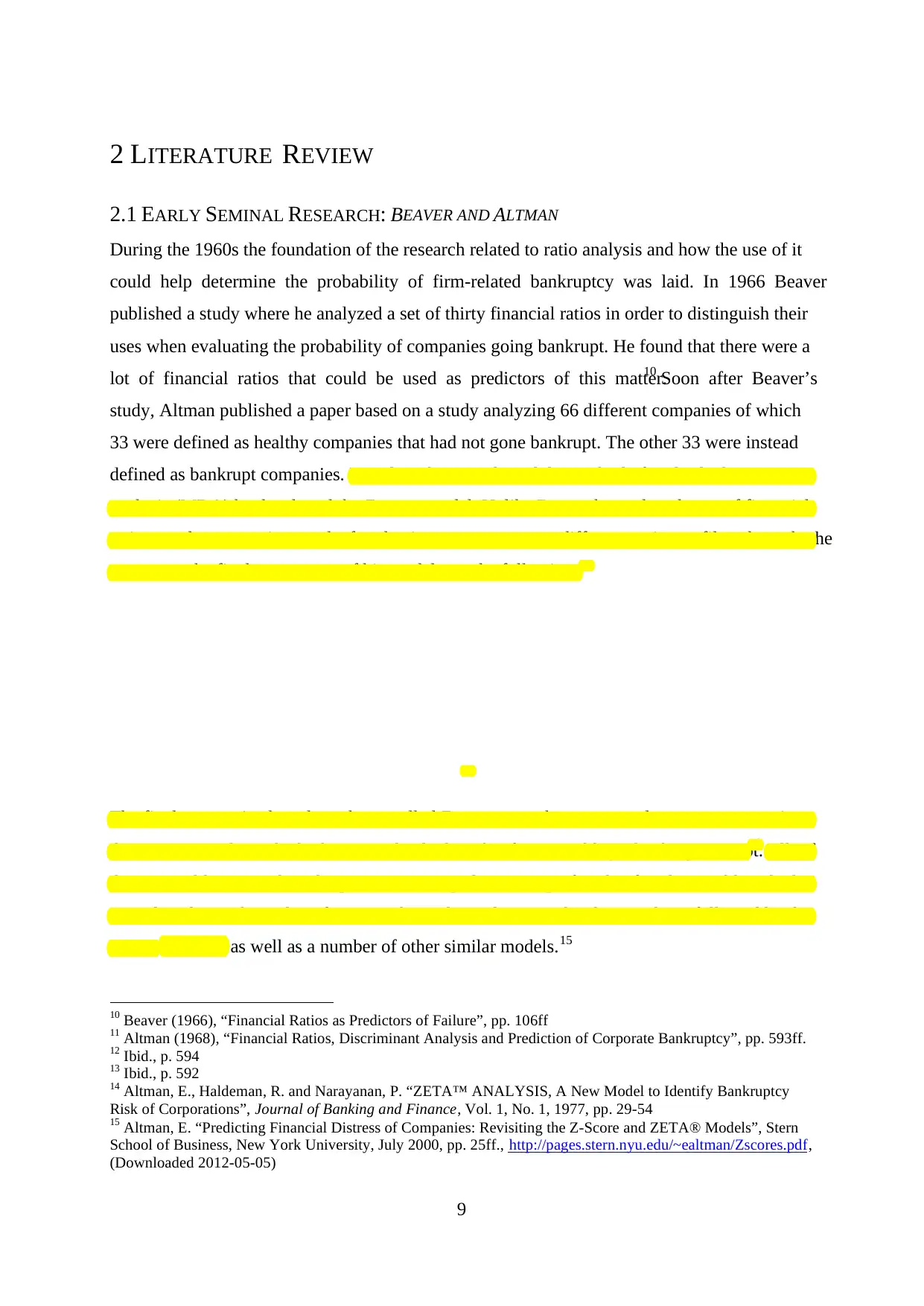
computer, the final appearance of his model was the following:11
12
The final summarized product, the so called Z-score, was then compared to an accompanying
discriminant value which determined whether the firm would go bankrupt or not.13 All of
these variables were based upon accounting data, except for the fourth variable which
considers the market value of equity. The traditional Z-score has later on been followed by the
ZETA model14, as well as a number of other similar models.15
10 Beaver (1966), “Financial Ratios as Predictors of Failure”, pp. 106ff
11 Altman (1968), “Financial Ratios, Discriminant Analysis and Prediction of Corporate Bankruptcy”, pp. 593ff.
12 Ibid., p. 594
13 Ibid., p. 592
14 Altman, E., Haldeman, R. and Narayanan, P. “ZETA™ ANALYSIS, A New Model to Identify Bankruptcy
Risk of Corporations”, Journal of Banking and Finance, Vol. 1, No. 1, 1977, pp. 29-54
15 Altman, E. “Predicting Financial Distress of Companies: Revisiting the Z-Score and ZETA® Models”, Stern
School of Business, New York University, July 2000, pp. 25ff., http://pages.stern.nyu.edu/~ealtman/Zscores.pdf,
(Downloaded 2012-05-05)

10
2.2 LOGIT MODELS: OHLSON
Apart from Beaver and Altman, an extensive array of studies have been conducted within this
research area and there are now a wide variety of models that have been developed and which
attempts to predict the bankruptcy of firms. The most important one regarding this study is the
one conducted by Ohlson, who presents a binary model. It is similar to Altman’s original Z-
score in the sense that it is meant to predict corporate failure as evidenced by the event of
bankruptcy. Another similarity is the almost exclusionary use of key ratios and accounting-
based information. However, this binary model uses a different statistical approach enabling a
more unhampered sample and sampling method. The statistical approach enabling this is the
logistic approach (or the logit approach) and Ohlson has, unlike Altman, not used a small
sample were failing companies and non-failing companies have been paired together. Instead
he has used a sample consisting of 105 failing companies and 2,058 non-failing companies,
all of which had been or was listed companies.16
Instead of five variables, like Altman’s Z-score model, 17 Ohlson’s so called O-score is
constituted out of nine variables, including both financial ratios and specific dummies
attempting to enhance predictability of his model. 18 Each variable is described below by the
words of Ohlson himself:
1. SIZE = log(total assets/GNP price-level index). The index assumes a base value of
100 for 1968. Total assets are as reported in dollars. The index year is as of the year
prior to the year of the balance sheet date. The procedure assures a real-time
implementation of the model. The log transform has an important implication.
Suppose two firms, A and B, have a balance sheet date in the same year, then the
sign of P A - P B is independent of the price-level index. (This will not follow unless
the log transform is applied.) The latter is, of course, a desirable property.
2. TLTA = Total liabilities divided by total assets.
3. WCTA = Working capital divided by total assets.
4. CLCA = Current liabilities divided by current assets.
5. OENEG = One if total liabilities exceeds total assets, zero otherwise.
6. NITA = Net income divided by total assets.
7. FUTL = Funds provided by operations divided by total liabilities.
16 Ohlson (1980), “Financial Ratios and the Probabilistic Prediction of Bankruptcy”, pp. 109f
17 Altman (1968), “Financial Ratios, Discriminant Analysis and Prediction of Corporate Bankruptcy”, p. 594
18 Ohlson (1980), “Financial Ratios and the Probabilistic Prediction of Bankruptcy”, pp. 118f

11
8. INTWO = One if net income was negative for the last two years, zero otherwise.
9. CHIN = (NIt – NIt-1)/(|NIt| + |NIt-1|), where NI is net income for the most recent
period. The denominator acts as a level indicator. The variable is thus intended to
measure change in net income.19
In his study he presented results for three different models, which sought to predict the
probability of bankruptcy one year in advance, two years in advance given that the firm did
not go bankrupt during the first year and either one or two years in advance. 20 However, it is
only the first model which is of interest in this study as it is devoted to analyzing the
probabilities of financial distress one year in advance. Ohlson’s first model was presented
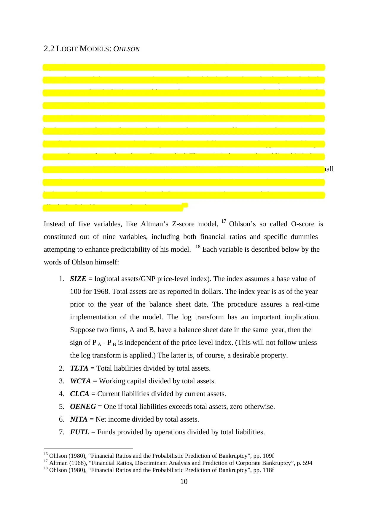
with the following appearance, describing the O-score:
21
Regarding the signs preceding these coefficients they could very well be logically explained
with regard to the essence of what these variables are trying to capture. This is however not
explained by Ohlson in his study. SIZE, WCTA, NITA, FUTL and CHIN are although ratios
that decreases the probability of failure, consequently presented as negative coefficients. As
the value they assume increase they are considered as being healthier, which is reflected in a
decreased probability of bankruptcy. OENEG is a variable trying to compensate for
companies whom present negative equity, or alternatively has total liabilities which are
exceeding total assets. This variable is by Ohlson described as neither truly negative nor truly
positive and its interpretation is thus not as clear-cut as for the others. TLTA, CLCA and
INTWO do understandably are positive coefficients, since a higher share of liabilities over
assets and a negative net income do not typically have a positive effect on a company’s well-
being. This means that they have an increasing effect on the probability of bankruptcy. 22
2.3 SWEDISH BANKRUPTCY PREDICTION MODELS: SKOGSVIK
Skogsvik has developed two models based upon a statistical method related to the logit
analysis – the probit analysis. His sample, aside from being Swedish, consists of industrial
companies with a data period ranging from 1966 to 1980. The observations were however
obliged to have had assets amounting to at least 200 million SEK or, as a minimum, 200
19 Ohlson (1980), “Financial Ratios and the Probabilistic Prediction of Bankruptcy”, pp. 118f
20 Ibid., p. 120
21 Ibid., p. 121
22 Ibid., p. 119

12
employees any year between 1966 and 1971. Comparable as to our study he defined the
failing firms, or the firms that had reached a state of financial distress, as either having gone
bankrupt, reached a composition agreement, voluntarily shut down the primary production
activity or received a receipt of a substantial subsidy provided by the state. His sample did
eventually contain 51 failing companies and 328 non-failing companies. 23 One of the models
was based upon current cost accounting (CCA), whilst the second one on the more commonly
used historical cost accounting (HCA) approach. This second one was intended to be used as
a reference model. The two models were developed independently and had slightly differing
sets of variables. 24 What he found was however that their performances were very alike, at
least as to their Type-I and Type-II error rates. 25 HCA ratios thus seemed to still prove to be
good predictors of business failure, in the sense that they have been employed earlier in the
studies of Beaver, Altman and Ohlson amongst others.26
2.4 RESEARCH CONSIDERING AUDIT REPORTS AND BANKRUPTCY
Auditing can be defined as “a systematic process of objectively obtaining and evaluating
evidence regarding assertions about economic actions and events to ascertain the degree of
correspondence between those assertions and established criteria and communicating the
results to interested users”.27 The results communicated to interested users are the audit
reports as well as the opinions derived from the financial statements of the company. The
most common opinion is an unmodified opinion, proclaiming that the statements are
presented fairly according to the auditor. If this is not the case, but rather that a modified
opinion is presented, there is probably something wrong with regards to the financial
statements and the accounting procedures of the company. It could be that the auditor has
found a material misstatement, but the company has refused to change it. It could also be that
the auditor has not been able to perform a satisfying evaluation. There can be several other
underlying reasons resulting in a modified opinion 28 and it is the relationship between these
reasons and bankruptcy which the following studies seek to undertake.
23 Skogsvik, K. “Current Cost Accounting Ratios as Predictors of Business Failure: The Swedish Case”, Journal
of Business Finance & Accounting, Vol. 17, No. 1, 1990, pp. 141f
24 Ibid., pp. 137f
25 Ibid., p. 152
26 Ibid., p. 138
27 Eilifsen, A., Messier, W., Glover, S. and Prawitt, D. Auditing & Assurance Services, 2nd revised ed., Berkshire:
McGraw-Hill Education, (2010), p. 10
28 Ibid., pp. 18-20

13
2.4.1 HOPWOOD , MCKEOWN & MUTCHLER
Regarding earlier research examining the relationship between audit reports and bankruptcies
there are many of whom that have proven its existence. The statements made by the auditor
could thus, to some extent, be used to foresee a bankruptcy. Hopwood et al. studied the
relationship between the audit reports and the financial failure of American companies. They
used one univariate test and two multivariate tests to examine this relationship. The univariate
test examined the dependence of the different kinds of opinions presented by the auditor. The
opinions were divided into three groups depending on whether they were related to
consistency, going-concern or other “subject-to” qualifications. All groups were proven to be
somewhat associated to bankruptcy.29
Regarding these groups and the different opinions; a consistency exception is attributable to a
change in accounting principles, a going-concern opinion refers to whenever an auditor have
doubts about the continued existence of an entity and a subject-to opinion is stated whenever
an auditor expresses uncertainties regarding something specific in the financial statements
which cannot be reasonably estimated and that is believed to have a material impact on the
appearance of the statements. The first multivariate test used the audit report variables in
conjunction with each other. It indicated a relationship between bankruptcy and both the
going-concern and other subject-to qualifications. In the second multivariate test the audit
report variables were jointly tested in a model together with a set of ratios that were solely
based upon accounting-based information. They then found that the consistency exception and
the going-concern opinions had incremental explanatory power. In relation to the ratios and
other subject-to opinions they did prove to have unique explanatory effects beyond these other
variables.30 They concluded the paper by stating that the study in fact does provide credence
to the use of auditors’ qualified opinions as an early warning signaling possible entity
failure.31
2.4.2 GAEREMYNCK & WILLEKENS
Gaeremynck & Willekens have also examined the relationship between audit reports and
company failure. Their definition of company failure included bankruptcies and voluntary
liquidations and the results which they presented in their study did point towards a strong
29 Hopwood, W., McKeown, J. and Mutchler, J. “A Test of the Incremental Explanatory Power of Opinions
Qualified for Consistency and Uncertainty”, The Accounting Review, Vol. 64, No. 1, 1989, p. 28
30 Ibid., pp. 29ff.
31 Hopwood et al. (1989), “A Test of the Incremental Explanatory Power of Opinions Qualified for Consistency
and Uncertainty”, p. 47

14
relationship between the two.32 The study they conducted was based upon 114 private Belgian
companies which had either become bankrupt or voluntarily liquidated in 1995 or 1996, as
well as a matched set of 114 healthy companies whose operations had not ceased during this
same time period. Both the financial statements and audit reports were subsequently analyzed.
Regarding the type of audit reports, out of this sample of 228 companies, they found that 155
had received a clean audit opinion, whilst the remaining 73 had received a non-clean audit
opinion. Out of these 73 non-clean audit reports, 62 belonged to the failing companies and
most of them (41 to be precise) pertained to the bankrupt companies. 33 The relationship was
also tested by the authors when performing a logistic regression analysis. The analysis
confirmed that there also was a statistical significance between the audit report opinion and
bankruptcy or voluntary liquidation.34
Other studies similar to these ones, also confirming there is a relationship between the
information provided by the audit report and company failure, have been carried out by
Altman & McGough and Sundgren.35 36
2.5 RELEVANT RECENT BACHELOR AND MASTER THESES
Similar studies, that have recently been performed and which we found interesting when
conducting this study first of all involve Andersson & Johansson. Their study is also heavily
influenced by the research done by Ohlson. However, they used another one of his models,
i.e. not the O-score. Nevertheless, they performed a logistic regression analysis evaluating the
performance of the model in predicting bankruptcies of Swedish non-listed companies. 37 As
part of their analysis they evaluated the error rate of Type-I and Type-II errors against a thesis
presented by Nyberg & Pesula who also employed a logistic regression analysis on
bankruptcies.38 However, their study primarily focused on the work made by auditors. Their
regression analysis emphasized what remarks had been made by the auditors, but they also
performed a test where financial key ratios were used collectively with the audit remarks.
32 Gaeremynck, A. and Willekens, M. “The Endogenous Relationship Between Audit-Report Type and Business
Termination: Evidence on Private Firms in a Non-Litigious Environment”, Accounting and Business Research,
Vol. 33, No. 1, 2003, p. 65
33 Ibid., pp. 72f.
34 Ibid., pp. 74ff.
35 Altman, E. and McGough T. “Evaluation of a Company as a Going Concern”, The Journal of Accountancy,
Vol. 138, No. 6, 1974, pp. 50-57
36 Sundgren, S. “Auditor choices and auditor reporting practices: evidence from Finnish small firms”, The
European Accounting Review, Vol. 7, No. 3, 1998, pp. 441-465
37 Andersson, A. and Johansson, H. “Prognostisering av Konkurs – En Logistisk Regressionsanalys av Svenska
Företag”, Företagsekonomiska Institutionen, Uppsala Universitet, 2009, pp. 15ff.
38 Ibid., p. 37

15
What their study pointed toward was a strong relationship between their factors (both key
ratios and audit-based variables) and the bankruptcies of these Swedish medium-sized
companies, studied in the thesis. 39 Kullerback & Löf has also made a study regarding
bankruptcy models and their uses related to Swedish firms. They used Altman’s Z-score to
evaluate its performance on a small sample of Swedish listed firms. However, their analysis
focused on the variables of the Z-score and the differences between them and the failing and
non-failing firms, as well as the outcome of the prediction results of the model.40
What all these theses do have in common is that they monitor Swedish firms, using the
insights of earlier studies made by some of the most notable researchers within this area. 41 42
43 The same goes for our study. However, ours still distinguishes itself by concentrating on
Ohlson’s O-score and Swedish listed firms, and at the same time employing an element of
auditing information. Our study could thus be considered to be partly influenced by these
studies, but by simultaneously displaying some other important and distinguishing features.
39 Nyberg, E. and Pesula, J. ”Revisionsberättelsen – är en användbar i en konkursförutsägelse?”, Institutionen för
företagsekonomi, Handelshögskolan i Umeå, Umeå Universitet, 2008, pp. 66f.
40 Kullerback, K. and Löf, M. ”Konkursanalys av bolag noterade på stockholmsbörsen - ett test av Edward I
Altmans Z-scoremodell”, Företagsekonomiska institutionen, Uppsala Universitet, 2008, pp. 15ff.
41 Andersson & Johansson (2009), “Prognostisering av Konkurs – En Logistisk Regressionsanalys av Svenska
Företag”, pp. 6ff.
42 Nyberg & Pesula (2008), ”Revisionsberättelsen – är en användbar i en konkursförutsägelse?”, pp. 9ff.
43 Kullerback & Löf (2008), ”Konkursanalys av bolag noterade på stockholmsbörsen - ett test av Edward I
Altmans Z-scoremodell”, p. 2

16
3 METHOD
As outlined above, this study focuses on analyzing data in order to draw scientific conclusions
and find empirical evidence concerning the prediction of financial distress, with a starting
point in Ohlson’s O-score. The perspective of the analysis is based upon the external
stakeholders, since the internal stakeholders often have access to more information about the
company, i.e. insider information. The information obtainable by the external stakeholders is
also often the same information that we have easily been able to acquire. This involves
financial reports, audit reports and data describing the national economic development.
When conducting the study a deductive approach has been used. The purpose and aim of the
study is to test and evaluate the statistical relationships between accounting-based information
and financial distress. The main focus is to test Ohlson’s O-score and its appliance to Swedish
listed firms. We further test how the incorporation of audit information affects the overall
performance of the model and its predictability related to financial distress. This could
however be argued to be a somewhat inductive approach as we merge the theories of Ohlson
and his O-score and the theories regarding the relationship between bankruptcy, financial
distress and the opinion of the audit report. It might just as well be argued to be strictly
deductive as the analysis originates from already existing theories which we try to apply
jointly, rather than to generate new theories based upon our empirics and analysis.
While the approach of the study is, at least mainly deductive, the methods of it are truly
quantitative. A considerable part of the time committed when performing the research, has
been devoted to managing the sample in such a way that it corresponds to the methods used
by Ohlson in his paper about the O-score.44 The sample is then used and tested via certain
statistical models to subsequently have its outcome analyzed. First follows the collection of
the data and managing of the sample and the focus group, i.e. the financially distressed
companies. Afterward follows more about the methods used to test the relationship between
the variables and financial distress.
3.1 THE SAMPLE
The data is originating from three different sources. Most of it has been gathered from the
Affärsdata database, which contains accounting information of Swedish companies based on
44 Ohlson (1980), “Financial Ratios and the Probabilistic Prediction of Bankruptcy”, pp. 109ff.

17
the financial statements. Information has also been extracted from Bureau van Dijk’s database
Orbis, including industry belongingness. From the Swedish Central Bureau of Statistics,
Statistiska Centralbyrån or SCB, we have collected information depicting the development of
the Swedish gross domestic product (GDP).
When formulating and creating the sample, we decided to use a couple of requirements or
restrictions for reasons more thoroughly described and discussed below. At the same time we
carefully describe the whole process of gathering the data and compiling the sample. The
requirements are compiled in a list below.
I. The firm should be listed on or have been delisted from the Aktietorget, Nordic
Growth Market (NGM) or Nasdaq OMX Stockholm stock exchanges.
II. The firm should be Swedish, possessing a Swedish organization identity number.
III. The firm should not be dissolved through a merger.
IV. The firm should not be dissolved by unidentified reasons.
V. The firm should not be operating within the financial sector.
VI. The firm should be able to present reports for at least three consecutive accounting
periods.
VII. The thirdly collected reporting period of each firm should end in the end of year
2000 or later.
VIII. The firm should display complete reports, making sure that the calculation of each
variable in the model is enabled.
As an initial step, we turned to Orbis to assemble a list containing the name, organization
identity number (organisationsnummer) and status of each and every firm listed on the
Aktietorget, Nordic Growth Market (NGM) and Nasdaq OMX Stockholm stock exchanges. In
order to achieve this we used stock exchanges as the search criteria and selected the
exchanges just mentioned. As we only wish to investigate Swedish firms, foreign firms listed
on these stock exchanges were not included. This way a list of 649 Swedish firms being listed
on or delisted from one of these exchanges was consequently compiled.
At this stage, the sample contains firms that have met the criterions of (I) being listed on or
delisted from one of the three stock exchanges and (II) having a Swedish organization
number. Since the objective is to examine firms in financial distress we have (III) not
included mergers. Seventeen observations were since dropped due to having merged, whilst
another six due to committing to an upcoming merger. The rationale is that the financial state

18
of these companies would have otherwise been complicated to determine, as the reasons and
circumstances behind the merger could be of a different nature than simply being related to
the financial shape of the acquired company. The acquirer could have other strategic reasons
for committing to the purchase. The required information related to this issue was sought out
by running the 649 identification numbers towards Affärsdata and its search tool identifying
certain “district court codes” (tingsrättskoder). The search items corresponding to a
completed merger and a merger in progress are 41 and 49, respectively. Another three
companies were excluded (IV) since they have been dissolved because of reasons not defined.
These were identified by the status search tool in Orbis, since there was no corresponding
district court code that could be utilized in Affärsdata. At this stage the sample consisted of
617 observations.
Furthermore, companies that are operating in the industries related to the financial sector
often distinguish themselves from others as to their structure, bankruptcy environment and
commonly used accounting regulations, rules and principles. This was also a criterion stated
by Ohlson. However, he also excluded utilities and transportation companies. 45 An attempt to
exclude these kinds of businesses has not been made in this study as we do not wish to neglect
such companies. It is rather only (V) the financial sector which we have chosen to exclude
since it is the industry considered to possess the most distinguishing features compared to
other industries. This was done by using our list of identification numbers and the Orbis
database to allocate and exclude all firms with a NACE rev. 2 index code in the range of 6400-
6600. A total of 57 firms were excluded in this phase, leaving 560 observations. There was
however a number of firms that did not have any specific industry codes registered. Hence,
we examined the Articles of Association and excluded all firms whose main area of
operations was related to the financial markets or who primarily worked with supplying
financial services. This resulted in the exclusion of one observation. There were however
another eighteen observations that did not display any industry codes. These companies were
not interpreted as mainly operating in the financial sector as we examined the Articles of
Association and were thus kept in the sample.
The remaining number of observations, i.e. 559 companies, was then supplied with
accounting data from Affärsdata. We used the modified list of identification numbers to seek
out the information needed to calculate the variables that constitute the O-score.
45 Ohlson (1980), “Financial Ratios and the Probabilistic Prediction of Bankruptcy”, p. 114

19
Consequently, we established a sample containing information on total assets, total equity,
current assets, current liabilities, net income and funds from operating activities for each
company. As this study also aims to take some concern towards the quality of the annual
accounts with regard to the auditor’s report, remarks from the auditor concerning the financial
reports were also extracted. This variable is defined via a coding system supplied by
Affärsdata with: “1” indicating that there was no remarks made by the auditor, “2” indicating
that there was remarks made by the auditor, “3” indicating no existing audit report and “4”
indicating that there was no remarks but rather a comment made by the auditor. The third
code was not observed for any company, consequently all firms had an audit report
accompanying their annual report. Together with this information and a Swedish real GDP
index denoting the year of 1968 as index 100, just like Ohlson,46 all variables were made
possible to calculate.
The Affärsdata database does only supply data for the four most recent accounting periods.
That is however sufficient for this study as our main priority is to determine the probability of
the firm reaching a state of financial distress approximately one year in advance. We did
however set up a requirement (VI) obligating each observation to have been active and
reported annual accounts for at least three consecutive accounting periods. If the firm was
considered reaching a state of financial distress, the same requirement was applied, however
prior to the period it reached this state. Hence, an additional nine observations were excluded.
It could also be mentioned that Ohlson did set up a similar requirement. He did also study
listed firms, but excluded those that had not been traded during a three-year period prior to the
date of bankruptcy.47
As a penultimate requirement, (VII) we controlled that each firm’s third reporting period
ended no earlier than in the very end of 2000. By doing so we separated all observations
whose data did not entirely relate to the year of 2000 or later, however disregarding whether
the accounting period did follow the calendar year or not. This was merely a capricious cut-
off point. No observations were however dropped due to this requirement. As a final step
(VII) we also decided to exclude each firm that, after calculating the variables of the model,
could not display values for each and every variable. These observations did, in other words,
not have sufficient data for us to completely calculate the O-score. At this stage one
observation was excluded due to insufficient data regarding the computation of the CLCA
46 Ohlson (1980), “Financial Ratios and the Probabilistic Prediction of Bankruptcy”, p. 118
47 Ibid., p. 114

20
variable and another sixteen for not displaying any values denoting the cash flow from
operations and thus preventing the assessment of the FUTL variable.
3.1.1 THE FOCUS GROUP
The concluding step in the data gathering and sample setup was to determine what firms
would be defined as being in, or had already reached a state of financial distress. For this
study we used a somewhat multifaceted, yet clear and unwavering definition when isolating
these firms. From Affärsdata we were able to identify a number of financially distressed firms
by running our modified list of identification numbers towards the database and pinning down
different district court codes indicating certain conditions related to financial instability.
From Orbis we were also able to determine what firms had recently defaulted on payments by
searching for their present status. We also used two of the Affärsdata codes related to
bankruptcy; 20 and 21 indicating a commenced bankruptcy process and bankruptcy,
respectively. A second pair of codes was related to a liquidation of the company; 31 and 32
indicating a finished liquidation process as well as one about to commence. A fifth code was
corresponding to a business reorganizations about to commence; 80. The distribution among
each reason of financial distress is denoted below in Table 1.
When deciding upon which states or district court codes that were to be included in the
definition of financial distress, the main purpose was to include such states that did imply a
situation where the future existence of the company would be at peril. As the future existence
of a company is at peril, investors are often exposed to a significant risk of losing their whole
investment as they are not prioritized in the liquidating process of the bankrupt company. The
second code, indicating bankruptcy, is however representing an absolute state where the
Type of Financial Distress Code N
Default on payments 9
Bankruptcy process has commenced 20 23
Bankruptcy process is finished 21 2
Liquidation is finished 31 1
Liquidation shall commence 32 7
Business reorganization shall commence 80 6
Firms in financial distress 48
T A B L E 1
Distribution of Financially Distressed Firms

21
company by many means has ceased to exist. This is also indicated by the third and sixth
code. The other codes do instead indicate a state of financial distress connected to instability
as a significant possibility of bankruptcy, liquidation or business reorganization has emerged.
A company defaulting on payments does also indicate a financially distressed company, as it
has failed to meet its debt obligations.
Furthermore, other district court codes do exist which would also have fitted our definition
and interpretation of financial distress. Of course, these were all reviewed and considered for
inclusion. However, including them would have added little to the study, since they were not
represented within the sample.
Below, in Table 2, the descriptive statistics of the whole sample is compiled with respect to
the different accounts used and derived from the financial statements. The data is mainly
derived from the latest accounting period, but net income from the second latest accounting
period is also collected in order to assess the last two variables of Ohlson’s model. The
statistics are further divided into two groups – the financially distressed firms, i.e. the focus
group and the other surviving firms. The data from the focus group is thus compiled of
accounting information related to the latest available accounting period before reaching a state
of financial distress.

22
3.2 STATISTICAL METHODS
Three distinctive features can be outlined as part of the analysis inherent in this study. First,
we analyzed how well Ohlson’s original model, the O-score, behaves in the context of our
sample. For this, no certain statistical tests were needed, except the percent correctly predicted
measure. Second, we established a revised model (Model A), based upon the same variables
inherent in Ohlson O-score.48 For this we needed to perform a logistic regression analysis.
This was conducted in Stata using the command for logistic regression and the coef option
(the logit command would have provided us with the same output), resulting in the
coefficients of the regression analysis being displayed. If not using this option the odds ratios
will instead be displayed. Third, we incorporate two dummy variables related to the audit
report as well as test this new model (Model B). The first variable (code 2 in Affärsdata
considering audit remarks) is denoting whether or not the auditor had assured (by reasonable
48 Ohlson (1980), “Financial Ratios and the Probabilistic Prediction of Bankruptcy”, pp. 118f.
Account N Median Mean Standard
Deviation Min Max 10th
percentile
90th
percentile
Net Income Y1 533 -914 225 237 1 568 247 -1 994 000 25 422 000 -54 910 189 800
Net Income Y2 533 -1 196 219 015 1 839 946 -2 239 000 33 774 000 -53 555 148 000
Total Assets Y1 533 136 591 3 666 263 17 082 687 91 239 336 000 8 865 4 323 000
Total Liabilities Y1 533 32 935 1 987 214 9 976 313 2 144 763 008 1 600 2 036 100
Total Equity Y1 533 84 202 1 679 050 7 450 952 -114 466 94 573 000 3 629 2 077 000
Current Assets Y1 533 37 318 951 280 5 556 434 55 93 198 000 1 651 837 200
Current Liabilities Y1 533 20 191 936 161 5 320 189 2 76 948 000 1 125 774 100
Working Capital Y1 533 4 474 15 120 4 271 853 -70 829 000 45 064 000 -126 251 334 900
Cash Flow from Operations Y1 533 -1 911 128 589 1 107 702 -6 650 000 13 686 000 -119 789 152 100
Net Income Y1 485 -383 250 264 1 641 865 -1 994 000 25 422 000 -45 627 201 400
Net Income Y2 485 -773 242 248 1 927 301 -2 239 000 33 774 000 -53 678 156 679
Total Assets Y1 485 155 894 4 017 740 17 871 234 994 239 336 000 10 538 5 596 000
Total Liabilities Y1 485 36 137 2 178 032 10 439 874 2 144 763 008 1 639 2 382 000
Total Equity Y1 485 95 758 1 839 708 7 793 216 -114 466 94 573 000 4 667 2 847 000
Current Assets Y1 485 45 000 1 042 522 5 817 469 55 93 198 000 1 856 963 000
Current Liabilities Y1 485 21 404 1 025 187 5 569 818 2 76 948 000 1 125 823 051
Working Capital Y1 485 6 107 17 335 4 478 651 -70 829 000 45 064 000 -134 235 369 400
Cash Flow from Operations Y1 485 -1 204 143 517 1 159 979 -6 650 000 13 686 000 -134 447 192 900
Net Income Y1 48 -8 726 -27 640 79 598 -425 400 213 404 -86 905 2 034
Net Income Y2 48 -4 982 -15 737 81 542 -313 815 393 000 -53 555 2 276
Total Assets Y1 48 30 382 114 889 182 295 91 647 100 3 309 539 900
Total Liabilities Y1 48 19 645 59 156 107 743 518 452 877 1 304 179 290
Total Equity Y1 48 10 018 55 733 104 198 -41 723 489 435 -4 314 228 474
Current Assets Y1 48 8 393 29 362 51 953 59 246 000 210 99 948
Current Liabilities Y1 48 9 635 36 621 64 666 518 299 100 1 110 114 534
Working Capital Y1 48 -893 -7 259 39 121 -114 475 100 074 -53 160 23 130
Cash Flow from Operations Y1 48 -7 964 -22 244 82 297 -477 700 169 580 -56 374 10 387
All Firms in SampleSurviving Firms
Focus Group
Data Summary for Sample
T A B L E 2
(Financially Distressed)

23
assurance) that there are no material misstatements related to the financial statements, whilst
the second one (code 4 in Affärsdata considering audit remarks) is denoting whether the
auditor did just leave a comment related to the accounting or financial reports. The second
variable is thus a lighter version, considering the flaws were deemed to be non-material. A
logistic regression analysis is once again performed to test this new model. All three models –
the O-score (Model 1), Model A and Model B – are then analyzed upon their predictive power
in relation to the established sample. We do also put some emphasis on the statistical
properties generated through the logistic regression analysis, used to generate Model A and
Model B. These include the Wald chi-square test, the pseudo R-squared and the z-statistics of
each independent variable. A likelihood ratio test is also used to examine the difference
between Model A and Model B. Another measure, mentioned earlier, is the percent correctly
predicted (PCP) measure, which tries to capture and establish a sense of the performance of
the model. The construction of this measure is rather intuitive, as it is estimated by calculating
how many of the estimated failures and non-failures that are correctly predicted out of the
whole sample.49
3.2.1 THE LOGISTIC REGRESSION
As this study attempts to analyze the O-score, it is simply natural to employ the logistic
regression, or the logit model. Ohlson mentioned several advantages of this econometric
methodology in comparison to the Multivariate Discriminant Analysis (MDA), which at the
time had been a very popular technique for predicting corporate bankruptcy. For one, he said
that the logit model does not require that the predictors are normally distributed. This property
enables the use of dummy independent variables. Furthermore, the output of this model is
fairly intuitive as it more clearly manifests the impact of each factor by providing either a
negative or positive sign preceding each coefficient. Another advantage is that the specific
matching procedures of MDA, which often are rather arbitrary, become unnecessary. 50 Grice
& Ingram further discuss the MDA approach and the early studies of Altman by performing
tests related to his original Z-score model. 51 Hillegeist et al. discourage the use of both the Z-
score and the O-score in favor of other market-based models – more specifically the Black-
49 Wooldridge, J. Introductory Econometrics, 4th ed., Mason, Ohio: South-Western Cengage Learning, 2008, p.
581
50 Ohlson (1980), “Financial Ratios and the Probabilistic Prediction of Bankruptcy”, pp. 111f
51 Grice, J. and Ingram, R. “Test of the Generalizability of Altman’s Bankruptcy Prediction Model”, Journal of
Business Research, Vol. 54, No. 1, 2001, p. 60

24
Scholes-Merton Probability of Bankruptcy (BSM-Prob). 52 However, this study is devoted to
the accounting-based model of Ohlson because of the simplicity of the model and its recently
mentioned advantages.
Regarding the model and the logit approach, Ohlson describes it as a logistic test where X i
denotes a vector of predictors for each observation. We also let β be a vector of unknown
parameters and P(Xt, β) denote the probability of bankruptcy for any given X and β. P is then
some probability function, 0 ≤ P ≤ 1. The logarithm of the likelihood of any specific outcome
is then given by:
53
In this setup, S 1 is the (index) set of bankrupt firms and S 2 is the set of non-bankrupt firms.
For any specified function P, the maximum likelihood estimates of β 1, β2 …, are obtained by
solving:
54
From this Ohlson stated the probability of bankruptcy as:
55
This further implies that P is increasing in y; and y is equal to log[P/(l — P)]. 56 As all β’s are
multiplied by their respective coefficient for each firm and the product of these are
summarized, a higher score will then indicate a higher probability of bankruptcy. A most
certain case of bankruptcy should thus assess a score corresponding to a probability equal to 1
(or 100%), whilst the other extreme will be a score resulting in a probability equal to 0 (or
0%).
3.2.2 THE WALD CHI-SQUARE TEST
The Wald test is used to test multiple exclusion restrictions for logit models. It has an
asymptotic chi-square distribution which the Wald statistic is compared against. A higher
52 Hillegeist, S., Keating, E., Cram, D. and Lundstedt, K. “Assessing the Probability of Bankruptcy”, Review of
Accounting Studies, Vol. 9, No. 1, 2004, p. 5
53 Ohlson (1980), “Financial Ratios and the Probabilistic Prediction of Bankruptcy”, p. 117
54 Ibid., pp. 117-118
55 Ibid., p. 118
56 Ibid.

25
Wald statistic will indicate a lower probability of the results of the model being due to
chance.57
3.2.3 THE LIKELIHOOD RATIO TEST
The likelihood ratio (LR) test is, in similarity with the Wald test, a way of testing exclusion
restrictions for logit models. The LR-test uses a similar concept as the F-test does in a linear
model. More specifically, the F-test measures the increase in the sum of squared residuals
when variables are dropped from the model. Hence, we can use the LR-test to evaluate
whether the two additional audit variables jointly improve the O-score. The test is based upon
a chi-square distribution and the difference in the log-likelihood functions of the unrestricted
model (Model B) and the restricted model (Model A). The notion is such that, because the
maximum likelihood estimation (MLE) maximizes the log-likelihood function, we usually
arrive at a smaller log-likelihood by dropping variables. At least the log-likelihood should not
increase. The same notion goes for the R-squared which also never can increase after one has
excluded one or some variables. However, in order to establish whether these two variables
are important we need to examine whether the decrease in log-likelihood is large enough. To
determine if the decrease is large enough we need to compare it towards a critical value.
Hence, we compare the likelihood ratio statistic, which is twice the difference between the
log-likelihoods,
towards the chi-square distribution. 58 However, when using Stata we can instead calculate the
p-value corresponding to the statistic. A low p-value indicates that by jointly adding the
variables inherent in the unrestricted model results in a statistically significant improvement
in the fit of the model.59
3.2.4 THE PSEUDO R-SQUARED – MCFADDEN ’S R-SQUARED
The typical R-squared is used as a goodness-to-fit measure, which provides an approximation
on how well future outcomes are to be estimated by the model. If we analyze the R-squared of
an OLS regression the interpretation is relatively straightforward as it measures how much of
the total variability that is accounted for by the model. If, for instance, a specific model attains
57 Wooldridge, Introductory Econometrics pp. 579f.
58 Ibid., p. 580
59 UCLA: Academic Technology Services. Stata FAQ – How can I perform the likelihood ratio, Wald, and
Lagrange multiplier (score) test in Stata?. http://www.ats.ucla.edu/stat/stata/faq/nested_tests.htm (Visited 2012-
04-26)

26
a R-squared of 0.5, the variables of the model predict 50% of the variability of the dependent
variable.60
The problem which accompanies the use of logistic models is that this typical R-squared
measure cannot be employed. A wide variety of similar measures has consequently been
developed and do essentially try to capture the same thing, i.e. the explanatory power of the
variables. One of these, so called, pseudo R-squared measures is the McFadden’s R-squared.
This is also the one which accompanies the output provided by Stata when running a logistic
regression. Even though this measure, alongside with other pseudo R-squareds, has its
limitations it can still be used to interpret the results. Its usages in this study, mostly circulates
around the simple notion that a higher pseudo R-squared is more desirable. Furthermore, as
one can observe when examining this R-squared, there are some similarities between it and
the likelihood ratio test.
As with the likelihood ratio test, denotes the log-likelihood of the unrestricted model.
on the other hand, is the log-likelihood function in the model with only the intercept. The
notion is thus such that, if these two log-likelihoods are equal to each other the covariates
have no explanatory power. This is rather similar to the typical R-squared measure.61
3.2.5 THE Z-STATISTICS
When utilizing Stata, the more common way of determining significance levels are through a
t-statistic. However, when for instance running a logistic regression through the software, the
significance levels are determined by a z-statistic that follows the standard normal
distribution. Despite the different distributions related to the t-statistics and the z-statistics, the
interpretations accompanying the assessments of the two statistics and their corresponding p-
values are the same.62
60 Wooldridge, Introductory Econometrics, p. 40
61 Ibid., pp. 581f.
62 Statacorp, Kristin MacDonald. One-sided tests for coefficients. 2011.
http://www.stata.com/support/faqs/stat/oneside.html (Visited 2012-04-26)

27
4 ANALYSIS
4.1 RATIOS AND BASIC RESULTS
The ratios used have been taken straight out from Ohlson’s study. The first model (Model A)
is a replica of Ohlson’s Model 1 where no changes have been made in terms of descriptive
variables.63 When presenting the second model (Model B), we once again use Ohlson’s nine
variables described above, but add the two new audit variables described below as variables
10 and 11:
10. REV_2 = One if the financial statements have remarks from the auditor (code 2 in
Affärsdata considering audit remarks), zero otherwise.
11. REV_4 = One if the financial statements have comments made by the auditor (code 4
in Affärsdata considering audit remarks), zero otherwise.
The signs of REV_2 and REV_4 should be positive considering that a remark or comment on
the financial statements by the auditor is not desirable and should thus have a negative impact
on the firm. More thoroughly explained, variable 10 denotes whether or not the auditor has
assured (by reasonable assurance) that there are no material misstatements and variable 11
whether the auditor did just leave a comment on the accounting or financial reports,
considering the flaws as non-material.
Table 3 shows a profile analysis where mean and standard deviation of the predictors for the
sample is presented. The results shown in this table are in all sense what we expect. First, it
supports the reasoning behind the signs of the coefficients. Second, it shows significant
differences in line with the expectations between the bankrupt and non-failing firms. We see
that the sample of bankrupt firms has both higher mean values for the variables TLTA, CLCA,
FUTL, INTWO, OENEG, REV_2 and REV_4 and lower mean values for SIZE, WCTA, NITA
and CHIN compared to the non-failing firms. This follows the logic that each predictor will
on average increase the predicted probability of financial distress for actual financially
distressed firms than for surviving firms. When comparing the profile analysis to the data
presented by Ohlson we experience a rough dimidiation of SIZE, ten folding of CLCA and
also a positive divergence of similar magnitude in FUTL. 64 We expect that the main
63 Ohlson (1980), “Financial Ratios and the Probabilistic Prediction of Bankruptcy”, pp. 118f.
64 Ibid.

28
explanation to this difference is due to the differences in sample and time period, but of
course this is only an assumption and there are many other plausible explanations such as
outliers, errors in data etc.
The estimates computed using the logistic regression analysis was done in two sets. Model A
predicts financial distress within one year using the same predictors as Ohlson. Model B also
predicts financial distress within one year but this time with all the previously described
predictors. A summary of the results of Model A and Model B is presented in Table 4 and in
order to make comparison easier, Ohlson’s Model 1 is presented alongside with the results. 65
65 Ohlson (1980), “Financial Ratios and the Probabilistic Prediction of Bankruptcy”, p. 121
Variable Mean Standard
Deviation Mean Standard
Deviation Mean Standard
Deviation
SIZE 6.533 2.429 6.705 2.411 4.794 1.880
TLTA 0.791 6.071 0.623 5.166 2.486 11.796
WCTA -0.0395 3.551 0.146 0.345 -1.912 11.728
CLCA 9.803 96.863 5.459 46.926 53.691 285.244
NITA -0.290 2.070 -0.176 1.247 -1.436 5.568
FUTL -4.953 87.650 -5.142 91.854 -3.040 8.389
INTWO 0.445 0.497 0.419 0.494 0.708 0.459
OENEG 0.0263 0.160 0.0144 0.119 0.146 0.357
CHIN -0.0284 0.640 -0.0095 0.639 -0.219 0.633
REV_2 0.0356 0.186 0.0103 0.101 0.292 0.459
REV_4 0.0844 0.278 0.0660 0.249 0.271 0.449
N 533 485 48
T A B L E 3
Profile Analysis
All Firms in Sample Surviving Firms
Focus Group
(Financially
Distressed)

29
SIZE TLTA WCTA CLCA NITA FUTL INTWO OENEG CHIN REV_2 REV_4 CONST
Ohlson (1980) Model 1
Estimates -0.407 6.03 -1.43 0.0757 -2.37 -1.83 0.285 -1.72 -0.521 - - -1.32
t-statistics -3.78 6.61 -1.89 0.76 -1.85 -2.36 0.81 -2.45 -2.21 - - -0.97
Model A
Estimates -0.282 -0.077 -1.13 0.00194 -0.279 0.00171 0.458 -0.789 -0.496 - - -1.08
z-statistics -3.39 -2.44 -2.64 2.67 -1.98 0.38 1.09 -0.74 -1.54 - - -1.56
Model B
Estimates -0.184 -0.0425 -0.844 0.00152 -0.165 0.00063 0.165 -1.03 -0.499 3.10 1.48 -1.93
z-statistics -2.10 -2.27 -1.78 1.57 -2.59 0.48 0.34 -1.22 -1.49 4.62 2.73 -2.63
McFadden's R-squared Percent Correctly Predicted
Ohlson (1980) Model 1 n/a 58.23
Model A 0.2033 92.50
Model B 0.2906 93.43
T A B L E 4
Prediction Results
Variable

30
Ohlson uses 2.00 as a limit for the absolute values of the t-statistics when classifying which
coefficients that are “statistically significant at a respectable level”, 66 Skogsvik uses 1.40 as a
limit for the absolute values of the t-statistics to classify which ratios to include in an iterative
estimation of his models, and in standpoint of the new estimation evaluate their significance. 67
Using Ohlson’s absolute limit of 2.00 we classify SIZE, TLTA, WCTA and CLCA as
significant coefficients in Model A. In Model B SIZE, TLTA, NITA, REV_2 and REV_4 are
classified as significant. If we use 1.40 as an absolute cut off point for the t-statistics, all
coefficients except FUTL, INTWO and OENEG are classified as significant in both Model A
and Model B. Ohlson reports a very high significance in TLTA, and also a higher value of the
coefficient than what we get in both Model A and Model B. This might simply be the result of
differing samples as Ohlson only uses industrial companies where the effect of leverage most
likely is a more homogenous factor compared to cross-industrial-samples where leverage
most reasonably can have different meanings for different industries. This is of course only a
possible explanation and is not presented as a fact in this case.
A way to compare the accuracy of the three different models is to use the statistics percent
correctly predicted which is calculated as the percent correctly predicted companies by the
models using a cutoff point of 0.5. This means that a company with a predicted probability of
failure greater than 0.5 will be classified as a predicted financially distressed company and a
company with a predicted probability lower than 0.5 will correspondingly be classified as a
predicted surviving company. For a cutoff point of 0.5 to be accurate it implicitly assumes a
symmetric relationship across Type-I and Type-II errors. Of course this is not the case, but it
is common practice to use this cutoff point for this type of measures.68 Table 4 shows the
percent correctly predicted and in order to evaluate these we must first specify that if all firms
were classified as surviving (a cutoff point of 0) the percent correctly predicted would equal
90.90 (485/533). This means that, if the percent correctly predicted for a model is less than
90.90 for this sample, one will on average have a higher percentage of correctly predicted
firms if one simply classifies all firms as not being financially distressed than if one uses the
model with the cutoff point of 0.5. Keeping this in mind and looking at the statistics presented
in Table 4 we clearly see that both Model A and Model B manages to beat 90.90 by a few
percentage points, but when we apply Ohlson’s Model 1 on our sample the percent correctly
66 Ohlson (1980), “Financial Ratios and the Probabilistic Prediction of Bankruptcy”, p. 120
67 Skogsvik (1990), “Current Cost Accounting Ratios as Predictors of Business Failure: The Swedish Case”, p.
143
68 Wooldridge, Introductory Econometrics, p. 581

31
predicted is as low as 58.23. Premature conclusions should not be drawn from this statistic;
this is only a measure that gives an indication of how well the model is fitted to the sample
and at most suggests that Ohlson’s Model 1 is not optimally adapted to the sample. However,
if we examine the results presented in Ohlson’s own study regarding this subject, the percent
correctly predicted for Model 1 amounts to 96.12. This value is also a few percentage points
above the limit describing the percent correctly predicted if all firms were classified as non-
bankrupt (equaling a cutoff point of 0). The limit Ohlson presents in his paper equals 91.15.
However, this limit appears to be subject to a miscalculation as his sample consists of 105
bankrupt firms and 2 058 non-bankrupt firms. This implies that the correct limit should be
95.15 . This further implies that our results are quite similar to his
results as to the percentages of correctly predicted observations gained by relying on the
models.69
Another way of determining how well the model and its predictors will describe the outcome
is by calculating the R-squared. As mentioned earlier the R-squared applicable for this kind of
studies is a pseudo R-squared and the one employed in this particular study is McFadden’s R-
squared. This pseudo R-squared is also used by Ohlson.70 The values of this measure vary
between zero and one. Since the first referral model where Ohlson’s Model 1 variables and
coefficients are used, is not directly derived from our sample no R-squared is reported.
However, the two other models, Model A and Model B are. Thus, their values are displayed
in Table 4. From Table 4 one can observe a rather significant difference between the two and
Model B assumes a much higher R-squared which should imply a higher predictability. It thus
seems as if the two audit variables, REV_2 and REV_4, do improve the model and provides
the model with important information. A second way, apart from the increased R-squared, to
determine the usefulness of these two added variables is to examine the Wald statistics. Also
these statistics suggest that the two variables contribute to the model. The Wald statistics for
Model A and Model B are 55.50 and 93.38, respectively. However, they both present p-values
very close to zero, indicating that the variables of each model are not simultaneously equal to
zero and thus contributing with a statistically significant improvement to the fit of the model,
compared with randomly assigning probabilities to each company regarding their likelihood
of reaching a state of financial distress in one year. A third way to test the reliability of these
two variables is to perform a likelihood ratio test comparing the extended (unrestricted)
69 Ohlson (1980), “Financial Ratios and the Probabilistic Prediction of Bankruptcy”, p. 120
70 Ibid., p. 121

32
Model B with (the restricted) Model A. The indication of this test is the same as of the R-
squared and Wald test. The likelihood ratio index amounted to 28.16 resulting in a p-value
close to zero, also implying a statistically significant improvement to the fit of the model.
There is thus substantial proof indicating that the audit information provided by these two
variables does increase the performance of the model. The improvement perhaps becomes the
most concrete and apparent from comparing the percent correctly predicted, however. As
described above, the indication is nonetheless the same.
To make sure that the coefficient groups of the audit variables (REV_2, REV_4), financial
state variables (SIZE, TLTA, WCTA, CLCA) and performance variables (NITA, FUTL,
INTWO, OENEG, CHIN) all contribute independently and significantly to the models, we
carry out an analysis of the correlation of the estimations presented in Table 5. The findings
are similar to those of Ohlson and supports that all variable groups are important in the
models.71 Furthermore, the correlation between the audit variables is as low as -0.06 which
indicates that these two variables do contribute significantly both jointly and independently.
We have done no attempts to change Ohlson’s variables or find any new existing accounting
predictors apart from the two audit variables. The idea with the model has always been that it
should be easy to use and that the information should be easily accessible. Tests were made
where we dropped variables with low significance (t-statistics lower than 1.40) but this
overall worsened the models predictability. If the addition of other variables would have
increased the models significance is unclear, but studies shows that market-based information
can be most useful in this context.72 Limitations in the collection of data has restrained us
form controlling for any market-based variables.
71 Ohlson (1980), “Financial Ratios and the Probabilistic Prediction of Bankruptcy”, pp. 122f.
72 Reisz, A. and Perlich, C. “A Market-Based Framework for Bankruptcy Prediction”, Journal of Financial
Stability, Vol. 3, No. 1, 2007, pp. 85f.

33
SIZE TLTA WCTA CLCA OENEG NITA FUTL INTWO CHIN REV_2 REV_4
SIZE 1
TLTA * 1
WCTA * -0.58 1
CLCA * * * 1
OENEG -0.25 0.41 -0.32 * 1
NITA * -0.23 -0.35 * -0.33 1
FUTL * * * * * * 1
INTWO -0.39 * * * * -0.21 * 1
CHIN * * * * * * * * 1
REV_2 -0.21 * -0.26 * 0.28 * * * * 1
REV_4 -0.23 * * * * * * 0.22 * -0.06 1
* = Absolute value of correlation is less than 0.20
T A B L E 5
Correlation Matrix of Estimations

34
4.2 EVALUATION OF PREDICTIVE PERFORMANCE
There is no standard procedure for when evaluating the accuracy of a bankruptcy prediction
model. The fact that there are two different types of errors (Type-I and Type-II) which cannot
be seen as simply additive to one another given that they are of somewhat different properties,
makes it even harder. On the other hand, looking at the model that has the lowest sum of
percentage errors is one of few possibilities to compare models. This type of comparison
cannot be seen as completely fair since the different models are often computed using
different samples, with different time periods, predictors, data, etc. Due to difficulties when
evaluating the model in any other way, this method of error minimization will be used, but we
will not make any cross model comparisons by given reasons.
All firms can fairly be divided into two groups by , estimated as financially distressed
or estimated as surviving, not financially distressed. This makes it interesting to present the
distribution of the estimated probabilities. Figure 1 shows the sample distribution one
year before financial distress for the 48 companies in the focus group using the estimated
coefficients from Ohlson’s Model 1. 73 Figure 2 and Figure 3 display the same distribution as
Figure 1, however instead using the estimated coefficients from Model A and Model B
respectively. The mean for each figure and their corresponding probabilities are 0.77, 0.26
and 0.36, respectively. Figure 4 shows the sample distribution for the 485 non-failing
firms, using the estimated coefficients from Ohlson’s Model 1. 74 In a similar fashion, Figure 5
and Figure 6 show the same using the estimated coefficients from Model A and Model B,
respectively. The distributions within the figures are grouped into two percentage intervals.
Furthermore, the mean for Figure 4, Figure 5 and Figure 6 and their corresponding
probabilities are 0.44, 0.07 and 0.06, respectively. The estimates related to Ohlson’s model
and its inherent coefficients are thus substantially larger than the estimates generated from our
Model A and Model B. This is apparent within the whole sample; hence the lower estimated
probabilities within both the failing and non-failing companies.
73 Ohlson (1980), “Financial Ratios and the Probabilistic Prediction of Bankruptcy”
74 Ibid.

35
0
10
20
30
40
50
0 0.1 0.2 0.3 0.4 0.5 0.6 0.7 0.8 0.9
Occurece (percentage)
Probability of Bankruptcy
F I G U R E 1
Probability Distribution of Focus Group (Financially Distressed) using
Ohlsons Model 1 Estimates
0
10
20
30
40
50
0 0.1 0.2 0.3 0.4 0.5 0.6 0.7 0.8 0.9
Occurece (percentage)
Probability of Bankruptcy
F I G U R E 2
Probability Distribution of Focus Group (Financially Distressed) using
Model A
0
10
20
30
40
50
0 0.1 0.2 0.3 0.4 0.5 0.6 0.7 0.8 0.9
Occurece (percentage)
Probability of Bankruptcy
F I G U R E 3
Probability Distribution of Focus Group (Financially Distressed) using
Model B

36
0
10
20
30
40
50
0 0.1 0.2 0.3 0.4 0.5 0.6 0.7 0.8 0.9
Occurece (percentage)
Probability of Bankruptcy
F I G U R E 4
Probability Distribution of Surviving Firms using Ohlsons Estimates
0
10
20
30
40
50
0 0.1 0.2 0.3 0.4 0.5 0.6 0.7 0.8 0.9
Occurece (percentage)
Probability of Bankruptcy
F I G U R E 5
Probability Distribution of Surviving Firms using Model A
0
10
20
30
40
50
0 0.1 0.2 0.3 0.4 0.5 0.6 0.7 0.8 0.9
Occurece (percentage)
Probability of Bankruptcy
F I G U R E 6
Probability Distribution of Surviving Firms using Model B

37
In order to classify errors for different cutoff points we examine the data underlying the
probability distribution models, in more detail. A Type-I error is defined as when a non-
failing firm has a probability greater than the cutoff point. A Type-II error is
consequently defined as when a bankrupt firm has a probability smaller than the
cutoff point. It would have been advantageous to perform this error analysis in an out-of-
sample test, which would probably have been helpful in either strengthening or rejecting the
models. Although, this was not possible to realize due to lack of data. We were neither able to
divide the sample in order to use one part for estimations and another for testing, because of
the size and ratio of financially distressed firms to surviving firms. Ohlson did not perform
any out-of-sample tests in his study, reasoning that this would not be a serious problem
considering that the sum of the percentage errors are quite stable over a wide range of cutoff
points. This turns out to be the case in our study as well. He also states that using a
sufficiently large sample should provide estimations which are not too sensitive to different
samples. Regarding the size of our sample, we will not make any claims regarding whether it
is sufficiently large as it is merely a fourth as big as Ohlson’s. On the other hand, our sample
is compiled from 533 observations and comprises a higher ratio of financially distressed
companies in comparison to the bankrupt firms used by Ohlson. Evidently these arguments
will be invalidated in a real-world application of the models, if the beta parameters are
considerably different in the application period.75
When Type-I and Type-II errors are expressed as percentages, they are tradeoffs to one
another. The cutoff points that minimize the percentage sum of errors are presented in Table
6. If there are X percent Type-I errors and Y percent Type-II errors at the cutoff point that
minimizes the sum of the error rates, the expected error rate is calculated as (X + Y) / 2, given
an infinite population where half of the firms are failing and the other half are non-failing.
75 Ohlson (1980), “Financial Ratios and the Probabilistic Prediction of Bankruptcy”, pp. 125f
Cutoff point Expected
Error Rate
Ohlson Model 1 (1980) 0.440 26.75%
Model A 0.050 28.07
Model B 0.066 22.58
T A B L E 6
Cutoff Point that Minimizes Expected Error Rate

38
The cutoff point that minimizes the expected error rate is substantially lower for Model A and
Model B compared to as when we use Ohlson’s estimates. This is not surprising considering
what was reported in the probability distribution diagrams above (Figure 1-6). We experience
a slight improvement of the expected error rates of our Model A and Model B compared to
when we used Ohlson’s estimates. On the other hand the results are not as low as in Ohlson’s
original study where he reports an expected error rate of 14.9 percent at a cutoff point at
0.038. The differences between the samples are most likely the reason to the difference in the
expected error rate and as Ohlson states. Thus, it is not reasonable to make a direct
comparison between the different models using this measure, considering that different
samples and definitions of bankruptcy often are used as well as variables and modeling
methods.76
Furthermore, Ohlson writes: “Moreover, the accountants' reports would have been of little, if
any, use. None of the misclassified bankrupt firms had a ‘going-concern qualification’ or
disclaimer of opinion. A review of the opinions revealed that eleven of these companies had
completely clean opinions, and the two that did not had relatively minor uncertainty
exceptions. Curiously, some of the firms even paid dividends in the year prior to bankruptcy.
Hence, if any warning signals were present, it is not clear what these actually were."77
Although, our findings are different and we would actually want to stress the importance of
the audit-based variables. Table 7 displays the ratio of Type-II errors and how many of the
firms that are wrongly estimated to survive and that has either a REV_2 or REV_4.
Interestingly we find that when we use Olson’s Model 1 estimates we almost do not
misclassify any of these firms, and even manage to capture substantially more of them than
what we do in model B where we control for them.
76 Ohlson (1980), “Financial Ratios and the Probabilistic Prediction of Bankruptcy”, p. 126
77 Ibid., p. 129

39
The rationale behind the very low Type-II error rates of Ohlson’s Model 1 presented below is
that it overall yields much higher estimated probabilities compared to Model A and Model B,
as discussed above. This occurs at the expense of a much higher Type-I error rate. In Table 8
the Type-I and Type-II errors are presented for some selected cutoff points.
Once again we can observe the tradeoff relationship between Type-I and Type-II errors. A
closer examination of Table 8 will show that Model A and Model B are essentially equivalent
at different cutoff points whereas Ohlson’s Model 1 has a higher Type-I error rate and a lower
Type-II error rate than Model A and B systematically throughout the different cutoff points.
Type II
errors REV_2* REV_4** Type II
errors REV_2 REV_4 Type II
errors REV_2 REV_4
0.00 0% 0% 0% 0% 0% 0% 0% 0% 0%
0.10 8.33 0 50.00 37.50 6 33.33 39.58 0 5.26
0.20 8.33 20.00 40.00 66.67 18.75 25.00 50.00 0 12.50
0.30 8.33 20.00 40.00 77.08 21.62 21.62 60.42 0 27.59
0.40 8.33 20.00 40.00 81.25 23.08 23.08 60.42 0 27.59
0.50 18.75 10.00 40.00 83.33 22.50 25.00 64.58 3.23 29.03
0.60 25.00 7.69 30.77 85.42 21.95 26.83 70.83 5.88 32.35
0.70 27.08 7.14 28.57 85.42 21.95 26.83 77.08 13.51 29.73
0.80 37.50 5.26 21.05 85.42 21.95 26.83 85.42 21.95 26.83
0.90 41.67 9.52 19.05 87.50 23.81 26.19 85.42 21.95 26.83
1.00 100 29.17 27.08 100 29.17 27.08 100 29.17 27.08
* Percent of Type-II errors where the wrongly estimated firm has a REV_2
** Percent of Type-II errors where the wrongly estimated firm has a REV_4
Estimates
from:
Cutoff point
Ohlson Model 1 (1980) Model BModel A
T A B L E 7
Type II errors with REV_2 or REV_4 for Selected Cutoff Points
Type I* Type II** Type I Type II Type I Type II
0.00 100% 0% 100% 0% 100% 0%
0.02 86.19 0.00 81.86 2.08 83.51 0
0.04 78.97 4.17 57.11 6.25 47.42 6.25
0.06 75.05 6.25 43.09 14.58 28.25 20.83
0.08 71.34 6.25 32.16 27.08 16.70 33.33
0.10 68.66 8.33 25.36 37.50 11.75 39.58
0.20 56.08 10.42 5.57 66.67 5.98 50.00
0.30 49.07 10.42 1.65 77.08 3.09 60.42
0.40 45.15 10.42 0.41 81.25 1.65 60.42
0.50 41.44 20.83 0 83.33 0.82 64.58
0.60 37.73 27.08 0 85.42 0.82 70.83
0.70 33.61 29.17 0 85.42 0.41 77.08
0.80 31.34 39.58 0 85.42 0 85.42
0.90 25.57 43.75 0 87.50 0 85.42
1.00 0 100 0 100 0 100
*Type I: predict bancruptcy; actual nonbankrupt.
*Type II: not predicted bancruptcy; actual bankruptcy.
T A B L E 8
Type I-Type II Analysis for Selected Cutoff Points
Ohlson Model 1 (1980) Model BModel AEstimates from:
Cutoff point

40
5 CONCLUSIONS
We have showed that when Ohlson’s Model 1 is used to predict financial distress of Swedish
listed firms, the estimated probabilities are generally large in comparison to the revised
models. We also show that Model A and Model B, which we have modeled ourselves, display
a slightly lower rate of errors and higher statistical significance, indicating that these models
can be used with preference to Ohlson's Model 1 when predicting financial distress of
Swedish listed firms. Furthermore, our results thus indicate that accounting information can
very well be used to predict financial distress among companies, which is line with studies
conducted by Altman and Ohlson among others. 78 79 80
Results drawn form Model B also implies that remarks or comments made by the auditors on
the financial statement add significant information in predicting the probability of financial
distress in the models presented. These results are also in line with earlier studies including
e.g. Hopwood et al. and Gaeremynck & Willekens.81 82
As Ohlson concludes in his study, we also believe that significant improvements of the
models presented, most likely require the addition of market-based predictors.83
78 Altman (1968), “Financial Ratios, Discriminant Analysis and Prediction of Corporate Bankruptcy”, p. 609
79 Altman et al. (1977), “ZETA™ ANALYSIS, A New Model to Identify Bankruptcy Risk of Corporations, pp.
49f.
80 Ohlson (1980), “Financial Ratios and the Probabilistic Prediction of Bankruptcy”, p. 130
81 Hopwood et al. (1989), “A Test of the Incremental Explanatory Power of Opinions Qualified for Consistency
and Uncertainty”, pp. 45ff.
82 Gaeremynck et al. (2003), “The Endogenous Relationship Between Audit-Report Type and Business
Termination: Evidence on Private Firms in a Non-Litigious Environment”, pp. 77f.
83 Ohlson (1980), “Financial Ratios and the Probabilistic Prediction of Bankruptcy”, p. 130

41
6 REFERENCES
PUBLISHED ARTICLES
Altman, E. “Financial Ratios, Discriminant Analysis and Prediction of Corporate
Bankruptcy”, Journal of Finance, Vol. 23, No. 4, 1968, pp. 589-609
Altman, E., Haldeman, R. and Narayanan, P. “ZETA™ ANALYSIS, A New Model to
Identify Bankruptcy Risk of Corporations”, Journal of Banking and Finance, Vol. 1, No. 1,
1977, pp. 29-54
Altman, E. and McGough T. “Evaluation of a Company as a Going Concern”, The Journal of
Accountancy, Vol. 138, No. 6, 1974, pp. 50-57
Beaver, W. 1966. “Financial Ratios as Predictors of Failure”, Journal of Accounting
Research, Vol. 4, No. 3, pp. 71-111
Gaeremynck, A. and Willekens, M. “The Endogenous Relationship Between Audit-Report
Type and Business Termination: Evidence on Private Firms in a Non-Litigious Environment”,
Accounting and Business Research, Vol. 33, No. 1, 2003, pp. 65-79
Grice, J. and Ingram, R. “Test of the Generalizability of Altman’s Bankruptcy Prediction
Model”, Journal of Business Research, Vol. 54, No. 1, 2001, pp. 53-61
Hillegeist, S., Keating, E., Cram, D. and Lundstedt, K. “Assessing the Probability of
Bankruptcy”, Review of Accounting Studies, Vol. 9, No. 1, 2004, pp. 5-34
Hopwood, W., McKeown, J. and Mutchler, J. “A Test of the Incremental Explanatory Power
of Opinions Qualified for Consistency and Uncertainty”, The Accounting Review, Vol. 64,
No. 1, 1989, pp. 28-48
Ohlson, J. “Financial Ratios and the Probabilistic Prediction of Bankruptcy”, Journal of
Accounting Research, Vol. 18, No. 1, 1980, pp. 109-131
Reisz, A. and Perlich, C. “A Market-Based Framework for Bankruptcy Prediction”, Journal
of Financial Stability, Vol. 3, No. 1, 2007, pp. 85-131
Skogsvik, K. “Current Cost Accounting Ratios as Predictors of Business Failure: The
Swedish Case”, Journal of Business Finance & Accounting, Vol. 17, No. 1, 1990, pp. 137-
160

42
Sundgren, S. “Auditor choices and auditor reporting practices: evidence from Finnish small
firms”, The European Accounting Review, Vol. 7, No. 3, 1998, pp. 441-465
NON-PUBLISHED ARTICLES
Altman, E. “Predicting Financial Distress of Companies: Revisiting the Z-Score and ZETA®
Models”, July 2000, http://pages.stern.nyu.edu/~ealtman/Zscores.pdf (Downloaded 2012-05-
05)
THESES
BACHELOR THESES
Andersson, A. and Johansson, H. “Prognostisering av Konkurs – En Logistisk
Regressionsanalys av Svenska Företag”, Företagsekonomiska Institutionen, Uppsala
Universitet, 2009
MASTER THESES
Kullerback, K. & Löf, M. ”Konkursanalys av bolag noterade på stockholmsbörsen - ett test av
Edward I Altmans Z-scoremodell”, Företagsekonomiska institutionen, Uppsala Universitet,
2008
Nyberg, E. and Pesula, J. ”Revisionsberättelsen – är en användbar i en konkursförutsägelse?”,
Institutionen för företagsekonomi, Handelshögskolan i Umeå, Umeå Universitet, 2008
LITERATURE
Eilifsen, A., Messier, W., Glover, S. and Prawitt, D. Auditing & Assurance Services, 2nd ed.,
Berkshire: McGraw-Hill Education, 2010
Wooldridge, J. Introductory Econometrics, 4th ed., Mason, Ohio: South-Western Cengage
Learning, 2008
INTERNET
SITES
UCLA: Academic Technology Services. Stata FAQ – How can I perform the likelihood ratio,
Wald, and Lagrange multiplier (score) test in Stata?.
http://www.ats.ucla.edu/stat/stata/faq/nested_tests.htm (Visited 2012-04-26)
Statacorp, MacDonald, K. One-sided tests for coefficients. 2011.
http://www.stata.com/support/faqs/stat/oneside.html (Visited 2012-04-26)

43
REPORTS
Tillväxtanalys, Konkurser och offentliga ackord 2011: Statistikrapport 2012:01, 2012-02-13,
http://www.tillvaxtanalys.se/tua/export/sv/filer/statistik/konkurser/Statistik_2012_01.pdf,
(Downloaded 2012-04-17)
NEWS ARTICLES
Rabe, M., ”Saab har problem – betalar inte underleverantörer”, Teknikens värld, 2011-03-29,
http://www.teknikensvarld.se/2011/03/29/12375/saab-har-problem--betalar-inte-
underleverantorer/, (Visited 2012-05-10)
TT, ”Saab går i konkurs”, Dagens Nyheter, 2011-12-19, http://www.dn.se/ekonomi/saab-
begars-i-konkurs, (Visited 2012-04-17)

44
APPENDIX A: SUMMARY OF THE FINANCIALLY DISTRESSED COMPANIES
Company ID Company Name Exchange NACE
Financial
Distress
Code
Last
available
report
Turnover Net
Income
Net
Income,
One Year
Prior
Assets Equity Current
Assets
Current
Liabilities
Cash Flow
from
Operations
SIZE
TLTA
WCTA
CLCA
OENEG
NITA
FUTL
INTWO
CHIN
REV_2
REV_4
5566768726 Allokton AB Delisted 6831 * 2010 21 192 213 404 -313 815 204 438 35 732 99 948 153 108 169 580 6.68 0.83 -0.26 1.53 0 1.04 1.01 0 1.00 0 1
5565560207 Alstrado AB Delisted 7320 * 2010 0 -3 018 -46 652 2 502 -13 967 2 502 16 469 -3 006 2.28 6.58 -5.58 6.58 1 -1.21 -0.18 1 0.88 1 0
5566850375 Ancora Energispar AB Delisted 2825 21 2007 32 715 -3 934 450 16 928 11 100 10 157 5 827 -8 929 4.19 0.34 0.26 0.57 0 -0.23 -1.53 0 -1.00 0 0
5565026563 Aqua Terrena International AB OMX - Nordic Exchange Stockholm 1107 * 2010 400 -8 730 -7 183 15 651 4 971 15 398 10 680 -6 999 4.11 0.68 0.30 0.69 0 -0.56 -0.66 1 -0.10 1 0
5561962035 Audiodev AB Delisted 2640 20 2008 88 260 -58 572 -44 310 154 892 99 751 118 005 55 141 -35 065 6.41 0.36 0.41 0.47 0 -0.38 -0.64 1 -0.14 0 0
5566609359 Bm Impex AB Delisted #N/A 20 2009 97 435 -1 706 -7 763 38 985 10 055 35 996 26 430 -2 457 5.08 0.74 0.25 0.73 0 -0.04 -0.08 1 0.64 0 0
5566603550 Brandworld Sverige AB (Publ) OMX - Nordic Exchange Stockholm 4642 80 2010 114 486 2 034 17 907 51 283 31 089 40 829 14 218 -14 380 5.30 0.39 0.52 0.35 0 0.04 -0.71 0 -0.80 0 0
5562474386 Catech AB Delisted 2849 20 2009 12 151 -2 304 3 492 21 927 9 871 4 350 2 419 -2 249 4.51 0.55 0.09 0.56 0 -0.11 -0.19 0 -1.00 0 0
5565523221 Catering Please I Skandinavien AB OMX - Nordic Exchange Stockholm 5610 * 2009 61 706 -7 628 -2 115 22 217 -2 268 12 365 18 485 -9 786 4.52 1.10 -0.28 1.49 1 -0.34 -0.40 1 -0.57 1 0
5566372636 Cellpoint Connect AB OMX - Nordic Exchange Stockholm 6190 * 2010 1 000 -44 958 -6 854 60 952 9 980 45 452 50 972 -56 374 5.47 0.84 -0.09 1.12 0 -0.74 -1.11 1 -0.74 1 0
5561534347 Cognos Technical Services AB Delisted #N/A 31 2008 62 244 57 154 16 948 135 564 98 505 134 079 34 005 -26 882 6.28 0.27 0.74 0.25 0 0.42 -0.73 0 0.54 0 1
5565418794 Countermine Technologies AB Delisted 2892 32 2009 2 712 -22 173 -8 266 287 600 258 226 93 041 24 783 -21 477 7.08 0.10 0.24 0.27 0 -0.08 -0.73 1 -0.46 1 0
5566069323 Dacke Group Nordic AB (Publ) Delisted #N/A 20 2008 4 948 -157 276 -170 516 60 873 -41 723 238 102 596 -143 545 5.48 1.69 -1.68 431.08 1 -2.58 -1.40 1 0.04 0 1
5566768254 Ekomarine AB (Publ) Delisted #N/A 20 2010 1 161 -8 721 -5 538 5 826 5 216 5 042 609 -9 209 3.12 0.10 0.76 0.12 0 -1.50 -15.10 1 -0.22 0 0
5566620570 Eriksson Development And Innovation Company AB Delisted 2811 * 2009 142 -2 244 -4 934 1 781 936 210 694 -1 911 2.00 0.47 -0.27 3.30 0 -1.26 -2.26 1 0.37 1 0
5566298914 Eurovip Group AB Delisted 7022 * 2010 125 -10 789 2 276 9 324 2 446 1 437 6 878 -12 031 3.60 0.74 -0.58 4.79 0 -1.16 -1.75 0 -1.00 0 1
5566400411 Fasttv Net AB Delisted 6020 80 2008 13 749 -37 706 -28 441 5 524 -14 456 4 016 19 980 -19 511 3.08 3.62 -2.89 4.98 1 -6.83 -0.98 1 -0.14 1 0
5562720358 Frontyard AB Delisted 6209 20 2003 5 648 -2 513 -26 841 38 847 18 979 1 870 6 655 -5 512 5.17 0.51 -0.12 3.56 0 -0.06 -0.28 1 0.83 0 0
5565490363 Gamers Paradise Holding AB Delisted 8292 20 2006 745 -86 905 -11 324 256 393 228 474 13 464 27 919 10 306 6.94 0.11 -0.06 2.07 0 -0.34 0.37 1 -0.77 0 0
5566802145 Gifttoday Sweden AB Delisted 4791 20 2009 6 148 -7 210 -3 272 11 534 4 734 1 857 4 211 -2 202 3.86 0.59 -0.20 2.27 0 -0.63 -0.32 1 -0.38 1 0
5565515938 Global Gaming Factory X AB OMX - Nordic Exchange Stockholm 7311 20 2009 3 560 -55 931 -856 3 309 -4 314 205 6 323 -53 909 2.62 2.30 -1.85 30.84 1 -16.90 -7.07 1 -0.97 0 1
5565837431 Globalfun AB Delisted 5829 20 2009 8 871 -4 714 55 7 938 2 031 3 955 4 778 -1 038 3.49 0.74 -0.10 1.21 0 -0.59 -0.18 0 -1.00 0 0
5562850098 Hebi Health Care AB Delisted 2120 20 2010 0 -32 099 -8 882 433 548 254 258 59 114 534 -21 913 7.43 0.41 -0.26 1941.25 0 -0.07 -0.12 1 -0.57 1 0
5563601821 Klippan AB Delisted 1712 20 2004 837 104 -54 910 -53 555 571 641 118 764 203 894 293 917 30 043 7.82 0.79 -0.16 1.44 0 -0.10 0.07 1 -0.01 0 0
5566280656 LayerlAB AB OMX - Nordic Exchange Stockholm 7211 * 2010 223 -3 280 -1 104 13 780 8 639 742 4 024 295 3.99 0.37 -0.24 5.42 0 -0.24 0.06 1 -0.50 0 0
5567022636 Metromark Hospitality Group AB (Publ) Delisted #N/A 20 2010 80 -37 349 -2 163 1 923 -2 785 1 923 3 058 -47 457 2.02 2.45 -0.59 1.59 1 -19.42 -10.08 1 -0.89 1 0
5565941787 Mfg Finance AB Delisted #N/A 32 2010 800 6 200 393 000 20 700 17 400 20 100 3 300 -169 200 4.39 0.16 0.81 0.16 0 0.30 -51.27 0 -0.97 0 0
5560226606 Micro Holding AB Delisted 4519 32 2008 4 276 51 400 60 155 58 851 14 999 1 304 -4 576 5.47 0.02 0.23 0.09 0 0.00 -3.51 0 -0.77 0 1
5565320537 Micus Sverige AB Delisted #N/A 20 2009 17 332 1 804 -572 10 866 2 488 6 040 5 266 4 881 3.80 0.77 0.07 0.87 0 0.17 0.58 0 1.00 0 1
5564354693 Nordic Electronic Procurement Systems AB OMX - Nordic Exchange Stockholm 6209 * 2010 2 035 1 587 -632 91 -7 387 91 7 478 1 -1.03 82.18 -81.18 82.18 1 17.44 0.00 0 1.00 1 0
5562110790 Novacast Technologies AB Delisted 6201 20 2009 10 544 -29 835 1 348 171 989 91 454 20 444 63 534 10 387 6.57 0.47 -0.25 3.11 0 -0.17 0.13 0 -1.00 0 0
5563785632 Obducat AB Nordic Growth Market (NGM) 2899 80 2010 10 233 -89 257 -51 549 43 124 20 771 3 100 22 353 -41 793 5.13 0.52 -0.45 7.21 0 -2.07 -1.87 1 -0.27 1 0
5565575965 Procast Media AB Delisted #N/A 80 2009 47 892 61 207 21 146 12 272 11 468 8 590 -1 592 4.47 0.42 0.14 0.75 0 0.00 -0.18 0 -0.54 0 0
5566263132 Pv Enterprise Sweden AB Delisted 2611 32 2010 349 724 -11 332 -27 662 99 618 33 896 58 864 55 552 7 586 5.96 0.66 0.03 0.94 0 -0.11 0.12 1 0.42 0 0
5566196993 Rayclinic AB Delisted 8610 20 2007 375 -13 536 -3 778 53 810 20 875 8 286 5 842 -13 008 5.35 0.61 0.05 0.71 0 -0.25 -0.39 1 -0.56 0 0
5567137947 Safe At Sea AB OMX - Nordic Exchange Stockholm 3012 80 2010 3 949 -2 970 -2 644 4 969 2 567 3 942 2 339 -2 341 2.97 0.48 0.32 0.59 0 -0.60 -0.97 1 -0.06 0 0
5564451655 Scanmining AB Delisted 2441 20 2006 156 217 -14 443 -22 875 543 346 489 435 44 541 21 411 -18 657 7.69 0.10 0.04 0.48 0 -0.03 -0.35 1 0.23 0 0
5566944954 Seanet Maritime Communications AB (Publ) Delisted 6190 80 2010 16 762 -29 328 -32 876 54 155 7 697 16 409 31 856 -13 024 5.35 0.86 -0.29 1.94 0 -0.54 -0.28 1 0.06 0 1
5566734835 Snowolverine Group AB Delisted 7490 32 2009 1 248 -15 713 -4 182 5 125 3 634 1 396 1 491 -18 687 3.05 0.29 -0.02 1.07 0 -3.07 -12.53 1 -0.58 0 1
5566092762 Stormfageln AB Delisted 3012 32 2009 88 -2 280 -2 230 10 303 8 883 146 1 109 -1 967 3.75 0.14 -0.09 7.60 0 -0.22 -1.39 1 -0.01 1 0
5565740064 Svithoid Tankers AB Delisted 5020 20 2007 4 100 2 600 -10 400 647 100 218 400 8 500 115 500 95 800 7.84 0.66 -0.17 13.59 0 0.00 0.22 0 1.00 0 0
5565425856 Tatura AB Delisted 7112 20 2008 125 -19 862 -11 318 38 547 19 126 14 565 7 896 -30 158 5.02 0.50 0.17 0.54 0 -0.52 -1.55 1 -0.27 1 0
5563987154 Teligent AB Delisted 6190 20 2007 262 800 -425 400 -142 300 539 900 167 000 246 000 299 100 -477 700 7.65 0.69 -0.10 1.22 0 -0.79 -1.28 1 -0.50 0 1
5564390341 Teligent Mobile Office AB Delisted 6201 32 2008 3 824 -200 078 -38 500 8 873 7 762 4 984 1 110 -25 721 3.55 0.13 0.44 0.22 0 -22.55 -23.15 1 -0.68 0 1
5561769596 Tivox AB Delisted 2849 21 2004 6 154 -27 440 -75 040 138 028 33 279 25 944 64 196 22 052 6.40 0.76 -0.28 2.47 0 -0.20 0.21 1 0.46 0 0
5562633098 Tmg International AB Delisted 4520 20 2006 169 -64 953 -4 481 595 690 324 829 42 008 26 075 -91 096 7.78 0.45 0.03 0.62 0 -0.11 -0.34 1 -0.87 0 1
5566819149 Trimera AB Delisted 2370 20 2009 773 -5 584 -1 020 6 291 5 773 4 994 518 -1 344 3.26 0.08 0.71 0.10 0 -0.89 -2.59 1 -0.69 0 1
5566329305 Xrf Analytical AB Delisted 5829 20 2009 675 -4 931 -5 030 5 665 1 944 1 513 3 277 -1 958 3.15 0.66 -0.31 2.17 0 -0.87 -0.53 1 0.01 0 0
All values are in thousands SEK
* Default of Payment