CSE6250: Big Data Analytics - Gradient Descent for Healthcare
VerifiedAdded on 2023/04/26
|6
|1063
|126
Homework Assignment
AI Summary
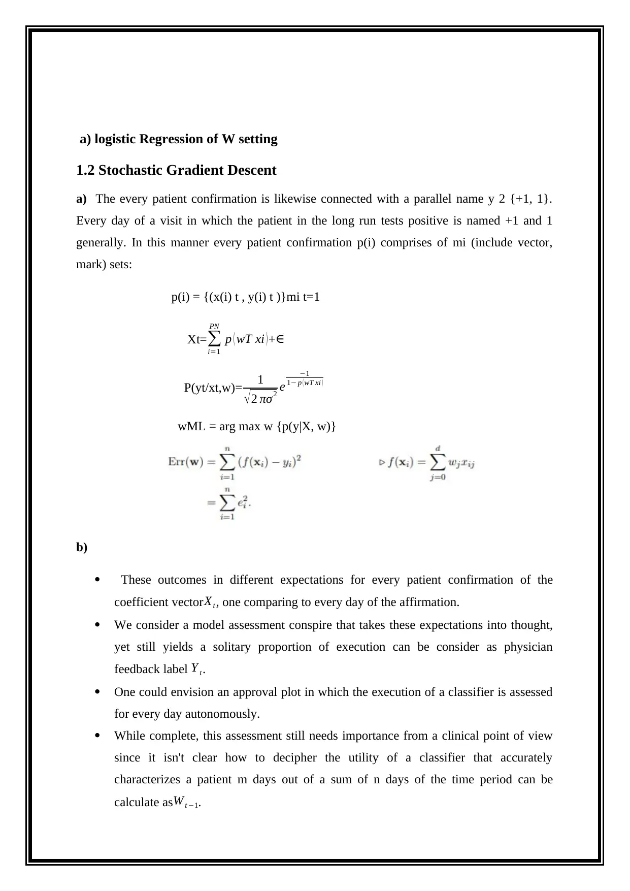
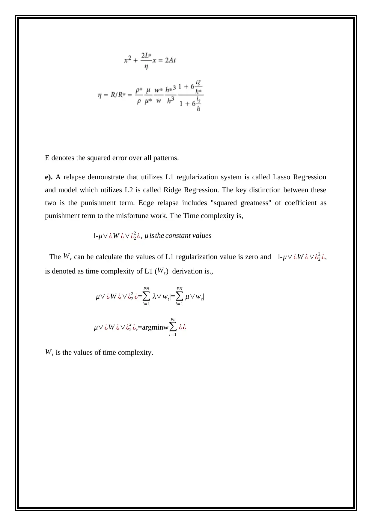
This assignment solution focuses on applying gradient descent methods, including batch and stochastic gradient descent, to a healthcare big data problem. It delves into the logistic regression of W setting, analyzes the time complexity of update rules, and discusses the impact of learning rates (η) on convergence. The solution also touches on L1 and L2 regularization techniques, such as Lasso and Ridge Regression, providing detailed derivations and explanations relevant to the CSE6250 Big Data Analytics in Healthcare course. The assignment aims to predict patient mortality using ICU clinical data, emphasizing the importance of accurate predictive analytics in healthcare.


1 out of 6


Your All-in-One AI-Powered Toolkit for Academic Success.
+13062052269
info@desklib.com
Available 24*7 on WhatsApp / Email
![[object Object]](/_next/static/media/star-bottom.7253800d.svg)
Copyright © 2020–2026 A2Z Services. All Rights Reserved. Developed and managed by ZUCOL.