Ask a question from expert
Bayesian Data Analytics (pdf)
14 Pages4150 Words209 Views
Added on 2022-01-21
Bayesian Data Analytics (pdf)
Added on 2022-01-21
BookmarkShareRelated Documents
1
Bayesian coursework specification for 2021
Data Analytics ECS648U/ ECS784U/ ECS784P
Revised on 25/02/2021 by Dr Anthony Constantinou and Dr Neville Kenneth Kitson.
1. Important Dates
• Release date: Thursday 25th February 2021 at 10:00 AM.
• Submission deadline: Wednesday, 28th April 2021 at 10:00 AM.
• Late submission deadline (cumulative penalty applies): Within 7 days after deadline.
General information:
i. When submitting coursework online you receive an automated e-mail as proof of
submission. Turnitin receipt does not constitute proof of submission. Some students
will sometimes upload their coursework and not hit the submit button. Make sure you
fully complete the submission process.
ii. A penalty will be applied automatically by the system for late submissions.
a. Your lecturer cannot remove the penalty!
b. Penalties can only be challenged via submission of an Extenuating
Circumstances (EC) form which can be found on your Student Support page.
All the information you need to know is on that page; including how to submit
an EC claim along with the deadline dates and full guidelines.
c. If you submit an EC form, your case will be reviewed by a panel and the panel
will make a decision on the penalty and inform the Module Organiser.
iii. If you miss both the submission deadline and the late submission deadline, you will
automatically receive a score of 0. Extensions can only be granted through approval
of an EC claim.
iv. Submissions via e-mail are not accepted.
v. It is recommended by the School that we set the deadline at 10:00 AM. Do not wait
until the very last moment to submit the coursework.
vi. Your submission should be a single PDF file.
vii. For more details on submission regulations, please refer to your relevant handbook.
2
2. Coursework overview
• The coursework is based on the Bayesian material and must be completed individually
(group submissions will not be accepted).
• To complete the coursework, follow the tasks below and answer ALL questions
enumerated in Section 3. It is recommended that you read the full document before you
start completing the tasks enumerated below.
• What follows has been tested on Windows and MAC operating systems. There is a
compatibility issue with MAC OS (and likely to extend to Linux) which is covered in
the Bayesys manual (details below), but which does not influence the coursework
submission requirements.
Task 1: Set up and reading
a) Visit http://bayesian-ai.eecs.qmul.ac.uk/bayesys/
b) Download the Bayesys user manual.
c) Set up the project by following the steps in Section 1 of the manual.
d) Read Section 2 of the manual.
e) Read Section 3.
f) Read Section 4.
g) Skip Section 5.
h) Read Section 6 and repeat the example.
i. MAC and Linux users will not be able to view the PDF graphs shown in Fig
6.1; i.e., the compatibility issue involves the PDF file generator.
ii. Skip subsections 6.3, 6.3.1, and 6.4.
i) Skip Section 7.
j) Skip Section 8.
k) Read Section 9.
l) Skip the appendices.
Task 2: Determine research area and collate data
You are free to choose or collate your own dataset. You should also determine the dataset
size, both in terms of the number of variables and the sample size, relevant to the problem
you are analysing. Some areas might require more data than others, and it is up to you to
make this decision.
3
You should address a data-related problem in your professional field or a field you are
interested in. If you are motivated in the subject matter the project will be more fun for you
and you will likely produce a better report. Section 5 provides a list of data sources you could
consider.
You are allowed to reuse the dataset you prepared during the Python coursework, as long as
a) your Python coursework submission was NOT a group submission, and b) you consider
the dataset to be suitable for Bayesian network structure learning (refer to Q1 in Section 3).
Lastly, you are not allowed to reuse datasets from the Bayesys repository for this
coursework.
Task 3: Prepare your dataset for structure learning
a) The Bayesys structure learning system assumes the input data are discrete; e.g.,
low/medium/high or Yellow/Blue/Green, rather than a continuous range of numbers.
If you have a continuous variable in your dataset with integers ranging, for example,
from 1 to 100, the algorithm will assume that this variable has 100 different states
(and many more if the values are not integer). This will make the dimensionality of
the model unmanageable, leading to poor accuracy and high runtime; if this is not
clear why, refer to the Conditional Probability Tables (CPTs) in the lecture slides and
relevant book material.
You should discretise continuous variables to reduce the number of states to
reasonable levels. For example, you could discretise the variable discussed above,
with values ranging from 1 to 100, into the five states {“1to20”, “21to40”, “41to60”,
“61to80”, “81to100”}. If a continuous variable incorporates a small number of
different values (e.g., less than 10), it may not need discretisation.
It is up to you to determine whether a variable requires discretisation, as well
as the level of discretisation. You are free to follow any approach you wish to
discretise the variable, including discretising the variables manually as discussed in
the above example. The structure learning accuracy is not expected to be strongly
influenced as long as the dimensionality of the data is reasonable with respect to its
sample size.
b) Your dataset must not have missing values (i.e., empty cells). Replace ALL empty
cells with the value ‘missing’ (or use a different relevant name). This forces the
algorithm to consider all missing values as an additional state. If missing data follows
a pattern, this may or may not help the algorithm to produce a more accurate graph.
c) Rename your dataset to trainingData.csv and place it in folder Input.
4
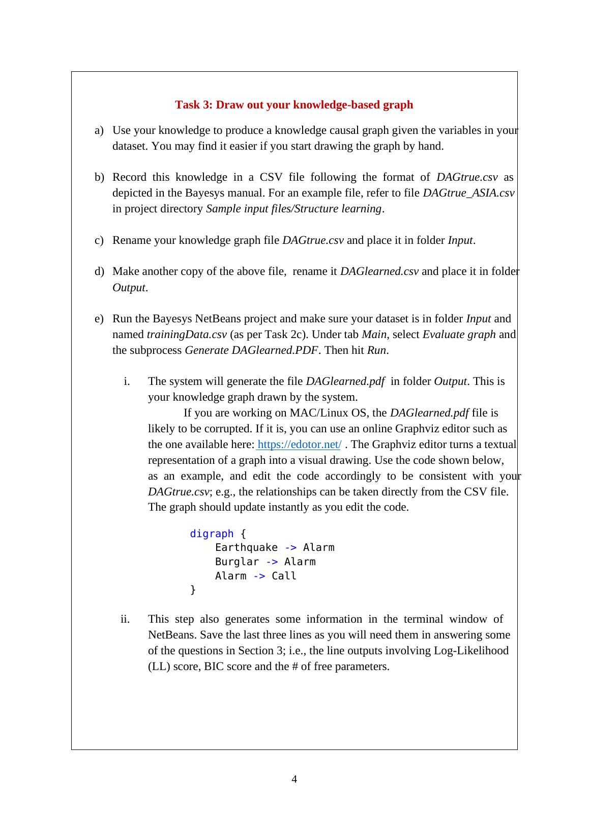
Task 3: Draw out your knowledge-based graph
a) Use your knowledge to produce a knowledge causal graph given the variables in your
dataset. You may find it easier if you start drawing the graph by hand.
b) Record this knowledge in a CSV file following the format of DAGtrue.csv as
depicted in the Bayesys manual. For an example file, refer to file DAGtrue_ASIA.csv
in project directory Sample input files/Structure learning.
c) Rename your knowledge graph file DAGtrue.csv and place it in folder Input.
d) Make another copy of the above file, rename it DAGlearned.csv and place it in folder
Output.
e) Run the Bayesys NetBeans project and make sure your dataset is in folder Input and
named trainingData.csv (as per Task 2c). Under tab Main, select Evaluate graph and
the subprocess Generate DAGlearned.PDF. Then hit Run.
i. The system will generate the file DAGlearned.pdf in folder Output. This is
your knowledge graph drawn by the system.
If you are working on MAC/Linux OS, the DAGlearned.pdf file is
likely to be corrupted. If it is, you can use an online Graphviz editor such as
the one available here: https://edotor.net/ . The Graphviz editor turns a textual
representation of a graph into a visual drawing. Use the code shown below,
as an example, and edit the code accordingly to be consistent with your
DAGtrue.csv; e.g., the relationships can be taken directly from the CSV file.
The graph should update instantly as you edit the code.
digraph {
Earthquake -> Alarm
Burglar -> Alarm
Alarm -> Call
}
ii. This step also generates some information in the terminal window of
NetBeans. Save the last three lines as you will need them in answering some
of the questions in Section 3; i.e., the line outputs involving Log-Likelihood
(LL) score, BIC score and the # of free parameters.
End of preview
Want to access all the pages? Upload your documents or become a member.
Related Documents
Bayesian Data Analytics (pdf)lg...
|14
|4155
|383
Southern Cross University (SCU) Assignment 2022lg...
|8
|2061
|20