Binge Drinking and Stroke for Young Adults

This study explores the association between binge drinking and stroke for young adults. Chi-square test of association was used to analyze the data. The study also calculates the proportion of stroke patients resulted from binge drinking and the number of patients to be given intervention to prevent 30 from binge drinking.

Binge Drinking and Stroke for Young Adults 1
BINGE DRINKING AND STROKE FOR YOUNG ADULTS
Name
Course Number
Date
Faculty Name

Binge Drinking and Stroke for Young Adults 2
Binge Drinking and Stroke for Young Adults
SECTION A
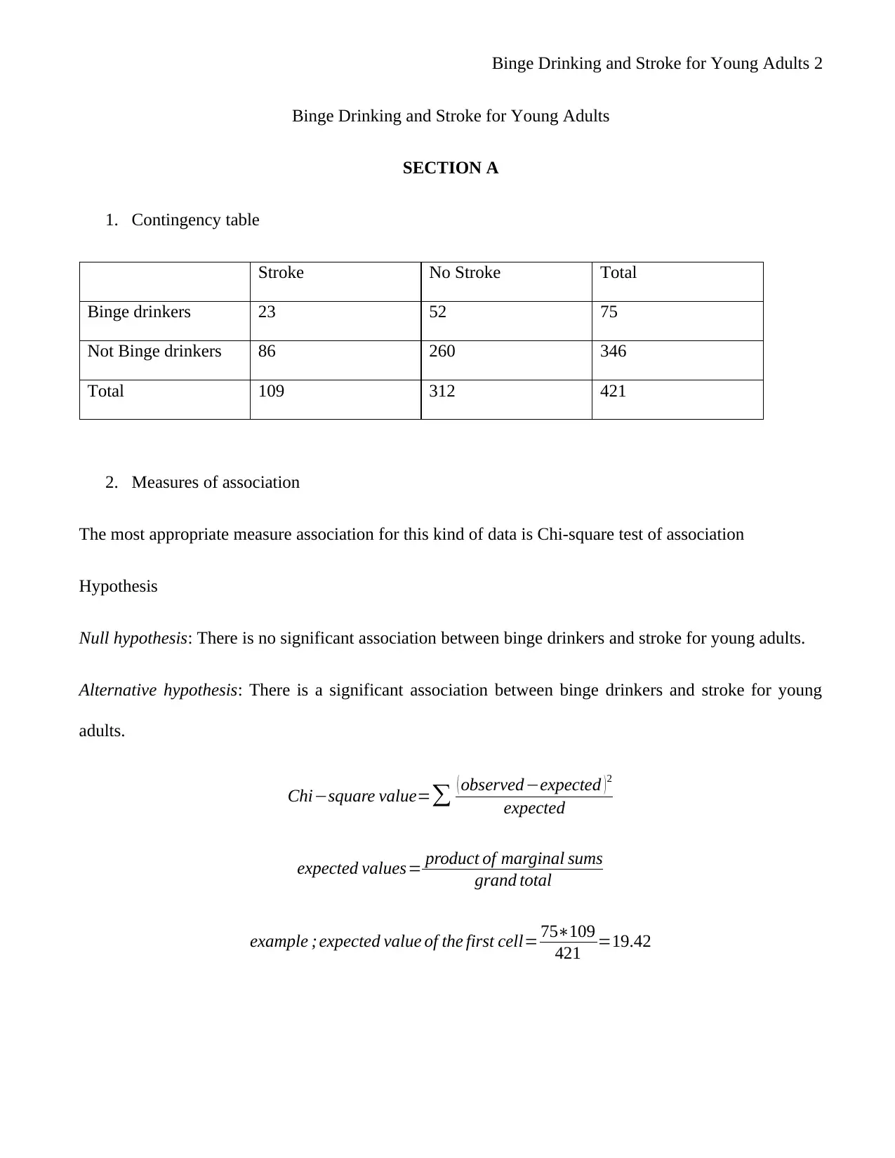
1. Contingency table
Stroke No Stroke Total
Binge drinkers 23 52 75
Not Binge drinkers 86 260 346
Total 109 312 421
2. Measures of association
The most appropriate measure association for this kind of data is Chi-square test of association
Hypothesis
Null hypothesis: There is no significant association between binge drinkers and stroke for young adults.
Alternative hypothesis: There is a significant association between binge drinkers and stroke for young
adults.
Chi−square value=∑ ( observed−expected ) 2
expected
expected values= product of marginal sums
grand total
example ; expected value of the first cell= 75∗109
421 =19.42

Binge Drinking and Stroke for Young Adults 3
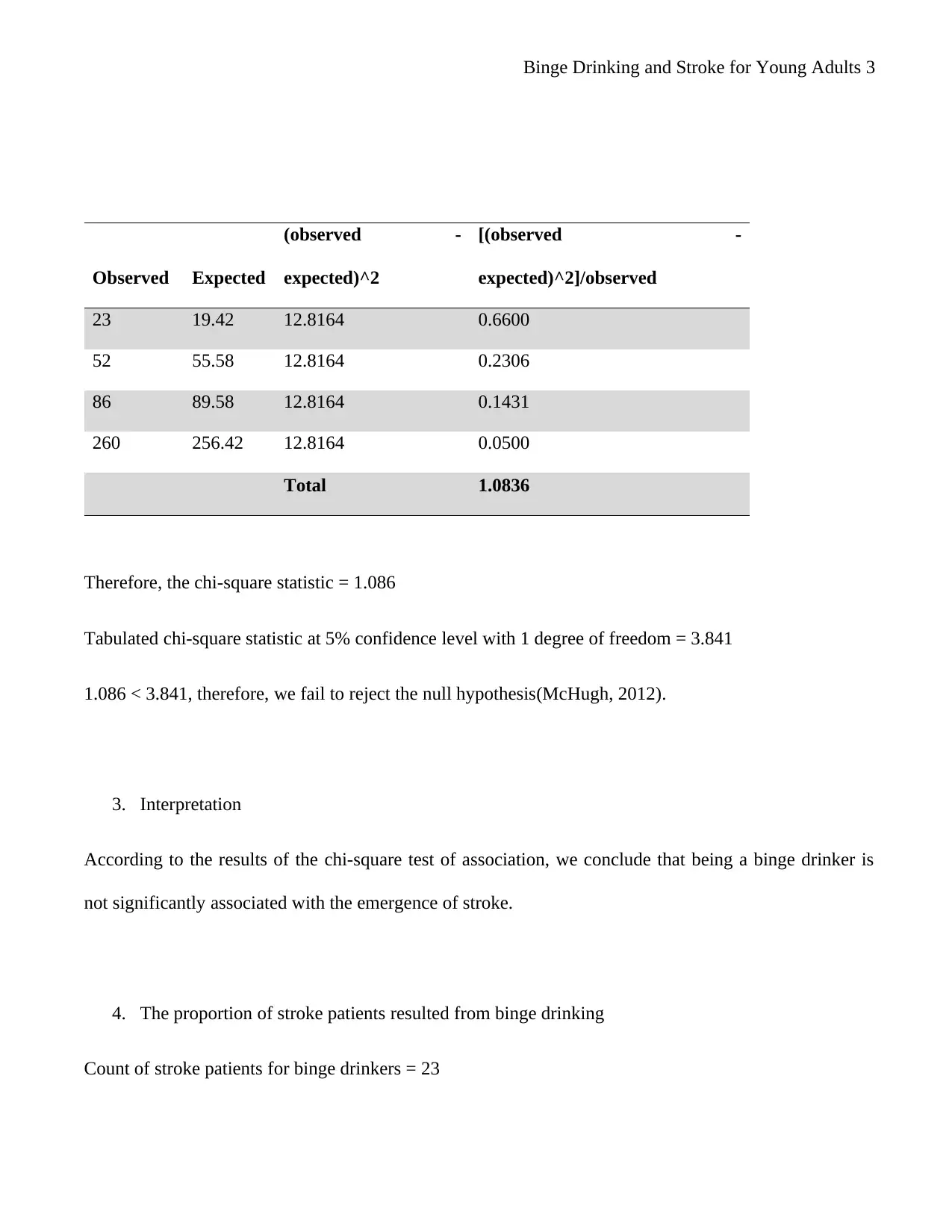
Observed Expected
(observed -
expected)^2
[(observed -
expected)^2]/observed
23 19.42 12.8164 0.6600
52 55.58 12.8164 0.2306
86 89.58 12.8164 0.1431
260 256.42 12.8164 0.0500
Total 1.0836
Therefore, the chi-square statistic = 1.086
Tabulated chi-square statistic at 5% confidence level with 1 degree of freedom = 3.841
1.086 < 3.841, therefore, we fail to reject the null hypothesis(McHugh, 2012).
3. Interpretation
According to the results of the chi-square test of association, we conclude that being a binge drinker is
not significantly associated with the emergence of stroke.
4. The proportion of stroke patients resulted from binge drinking
Count of stroke patients for binge drinkers = 23

Binge Drinking and Stroke for Young Adults 4
Count of stroke patients for non-binge drinkers = 86
Total number of stroke patients = 23 + 86 = 109
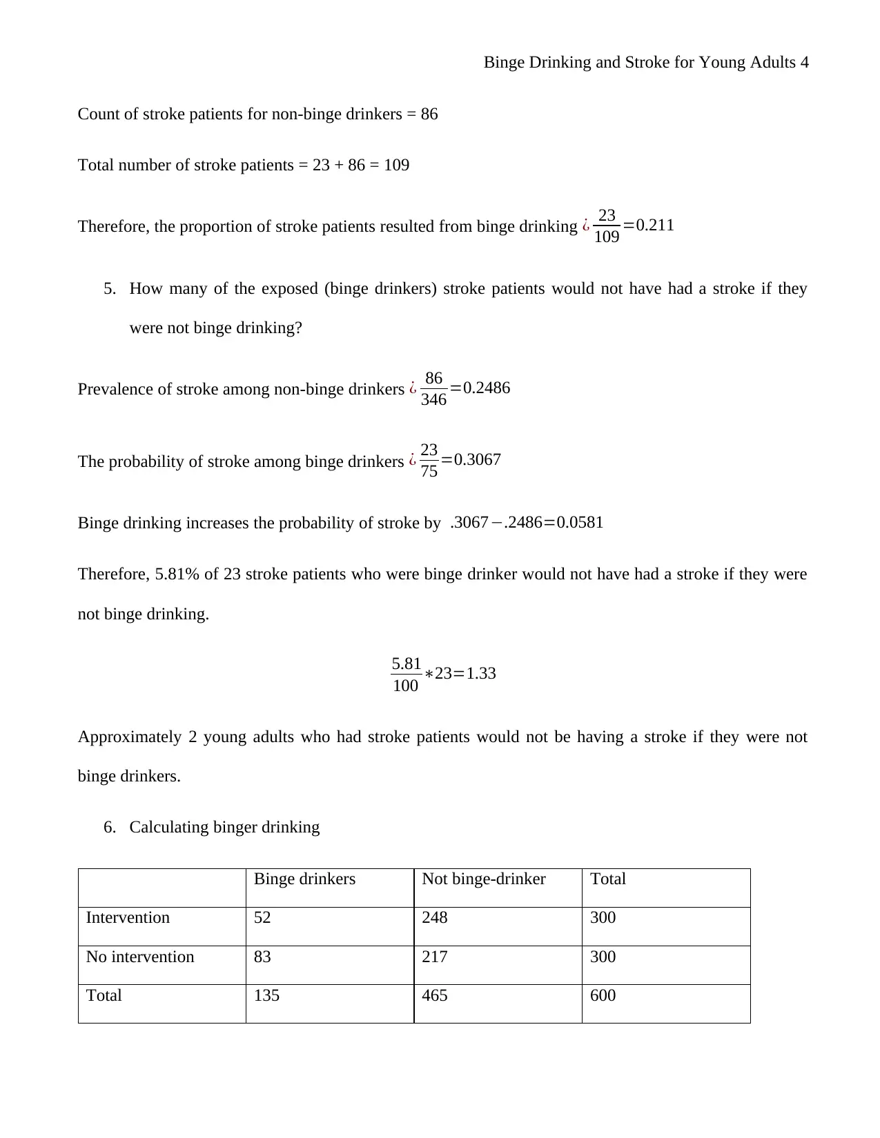
Therefore, the proportion of stroke patients resulted from binge drinking ¿ 23
109 =0.211
5. How many of the exposed (binge drinkers) stroke patients would not have had a stroke if they
were not binge drinking?
Prevalence of stroke among non-binge drinkers ¿ 86
346 =0.2486
The probability of stroke among binge drinkers ¿ 23
75 =0.3067
Binge drinking increases the probability of stroke by .3067−.2486=0.0581
Therefore, 5.81% of 23 stroke patients who were binge drinker would not have had a stroke if they were
not binge drinking.
5.81
100 ∗23=1.33
Approximately 2 young adults who had stroke patients would not be having a stroke if they were not
binge drinkers.
6. Calculating binger drinking
Binge drinkers Not binge-drinker Total
Intervention 52 248 300
No intervention 83 217 300
Total 135 465 600

Binge Drinking and Stroke for Young Adults 5
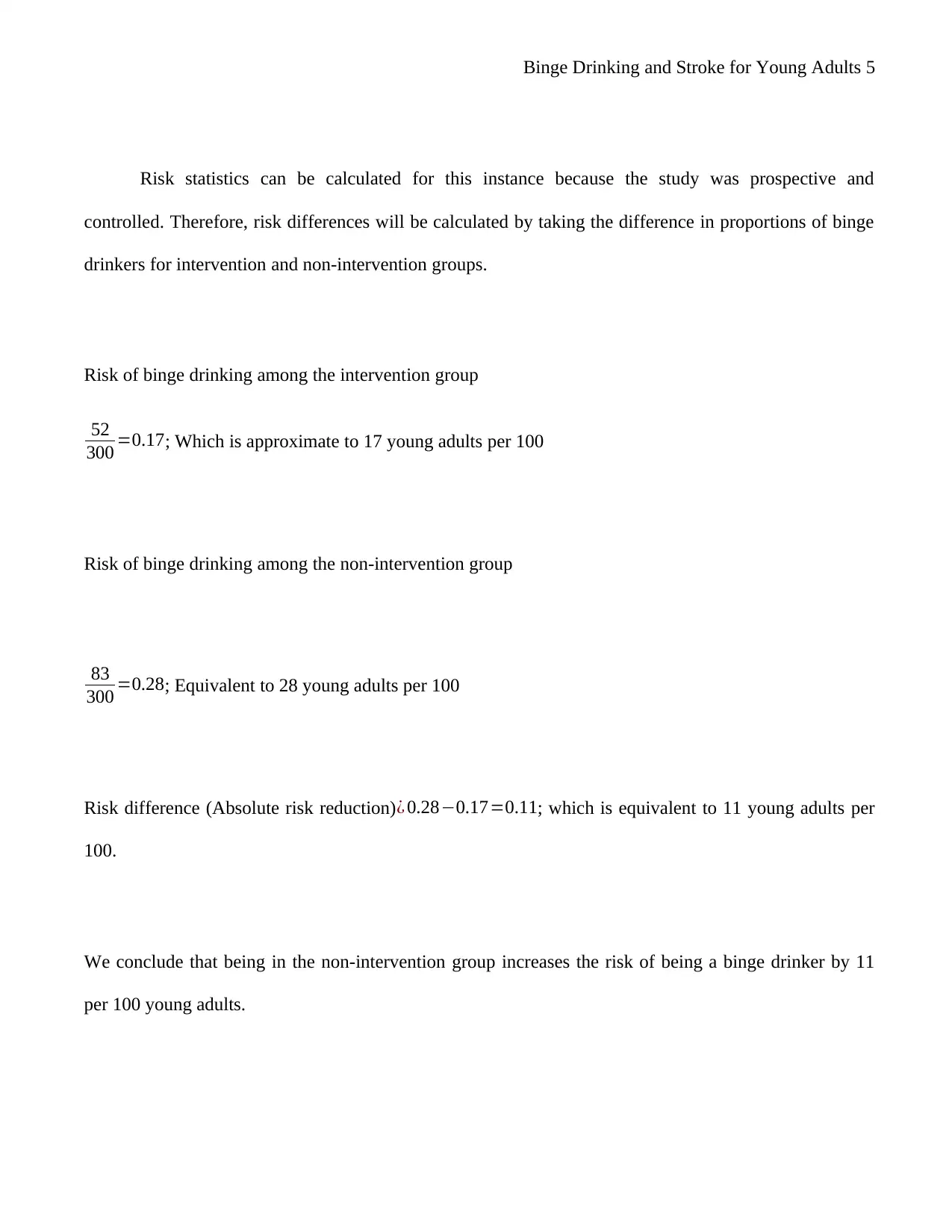
Risk statistics can be calculated for this instance because the study was prospective and
controlled. Therefore, risk differences will be calculated by taking the difference in proportions of binge
drinkers for intervention and non-intervention groups.
Risk of binge drinking among the intervention group
52
300 =0.17; Which is approximate to 17 young adults per 100
Risk of binge drinking among the non-intervention group
83
300 =0.28; Equivalent to 28 young adults per 100
Risk difference (Absolute risk reduction)¿ 0.28−0.17=0.11; which is equivalent to 11 young adults per
100.
We conclude that being in the non-intervention group increases the risk of being a binge drinker by 11
per 100 young adults.

Binge Drinking and Stroke for Young Adults 6
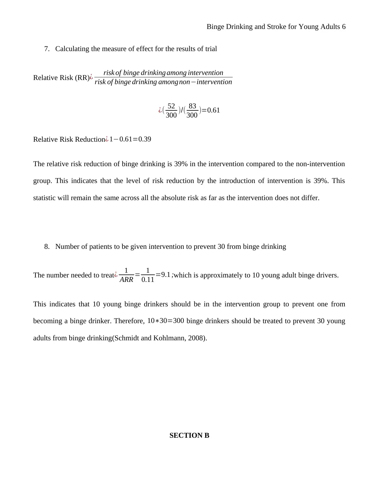
7. Calculating the measure of effect for the results of trial
Relative Risk (RR)¿ risk of binge drinking among intervention
risk of binge drinking amongnon−intervention
¿( 52
300 )/( 83
300 )=0.61
Relative Risk Reduction ¿ 1−0.61=0.39
The relative risk reduction of binge drinking is 39% in the intervention compared to the non-intervention
group. This indicates that the level of risk reduction by the introduction of intervention is 39%. This
statistic will remain the same across all the absolute risk as far as the intervention does not differ.
8. Number of patients to be given intervention to prevent 30 from binge drinking
The number needed to treat¿ 1
ARR = 1
0.11 =9.1 ;which is approximately to 10 young adult binge drivers.
This indicates that 10 young binge drinkers should be in the intervention group to prevent one from
becoming a binge drinker. Therefore, 10∗30=300 binge drinkers should be treated to prevent 30 young
adults from binge drinking(Schmidt and Kohlmann, 2008).
SECTION B

Binge Drinking and Stroke for Young Adults 7
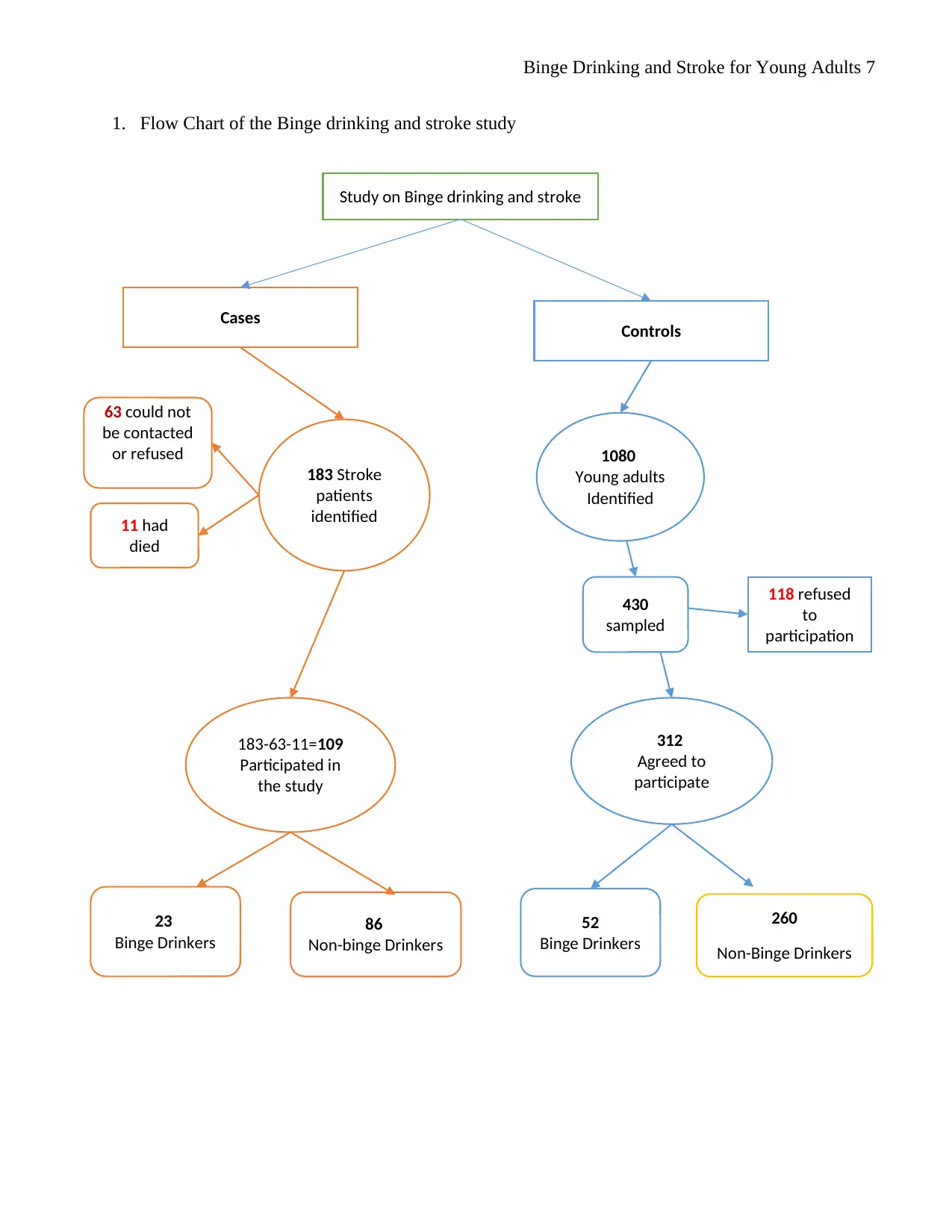
1. Flow Chart of the Binge drinking and stroke study
Study on Binge drinking and stroke
Cases
183-63-11=109
Participated in
the study
86
Non-binge Drinkers
23
Binge Drinkers
183 Stroke
patients
identified
63 could not
be contacted
or refused
11 had
died
312
Agreed to
participate
52
Binge Drinkers
Controls
1080
Young adults
Identified
430
sampled
118 refused
to
participation
260
Non-Binge Drinkers

Binge Drinking and Stroke for Young Adults 8
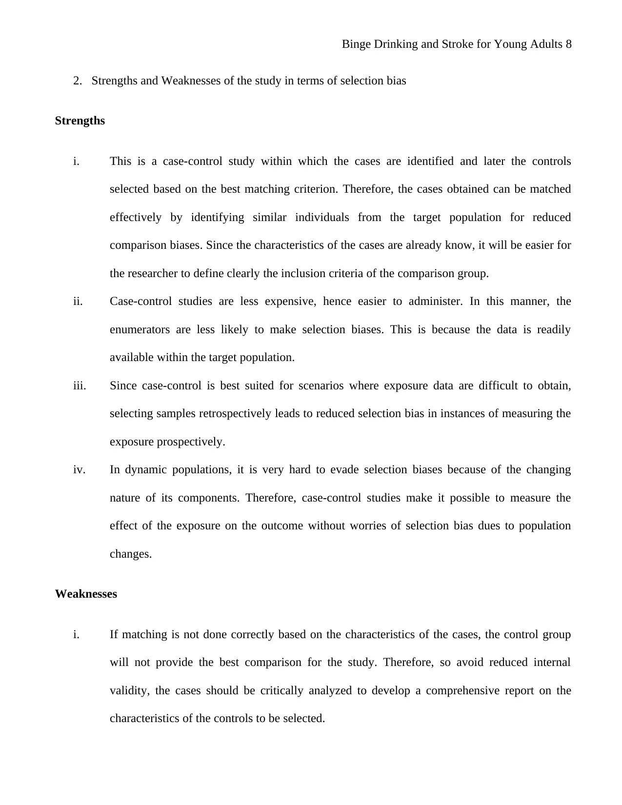
2. Strengths and Weaknesses of the study in terms of selection bias
Strengths
i. This is a case-control study within which the cases are identified and later the controls
selected based on the best matching criterion. Therefore, the cases obtained can be matched
effectively by identifying similar individuals from the target population for reduced
comparison biases. Since the characteristics of the cases are already know, it will be easier for
the researcher to define clearly the inclusion criteria of the comparison group.
ii. Case-control studies are less expensive, hence easier to administer. In this manner, the
enumerators are less likely to make selection biases. This is because the data is readily
available within the target population.
iii. Since case-control is best suited for scenarios where exposure data are difficult to obtain,
selecting samples retrospectively leads to reduced selection bias in instances of measuring the
exposure prospectively.
iv. In dynamic populations, it is very hard to evade selection biases because of the changing
nature of its components. Therefore, case-control studies make it possible to measure the
effect of the exposure on the outcome without worries of selection bias dues to population
changes.
Weaknesses
i. If matching is not done correctly based on the characteristics of the cases, the control group
will not provide the best comparison for the study. Therefore, so avoid reduced internal
validity, the cases should be critically analyzed to develop a comprehensive report on the
characteristics of the controls to be selected.

Binge Drinking and Stroke for Young Adults 9
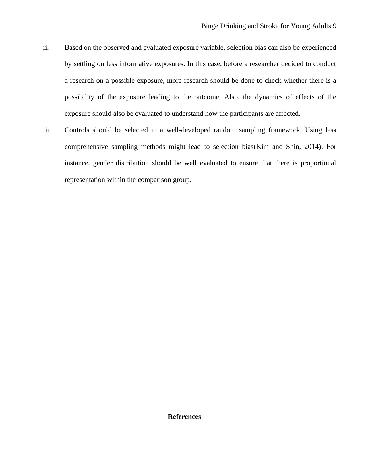
ii. Based on the observed and evaluated exposure variable, selection bias can also be experienced
by settling on less informative exposures. In this case, before a researcher decided to conduct
a research on a possible exposure, more research should be done to check whether there is a
possibility of the exposure leading to the outcome. Also, the dynamics of effects of the
exposure should also be evaluated to understand how the participants are affected.
iii. Controls should be selected in a well-developed random sampling framework. Using less
comprehensive sampling methods might lead to selection bias(Kim and Shin, 2014). For
instance, gender distribution should be well evaluated to ensure that there is proportional
representation within the comparison group.
References

Binge Drinking and Stroke for Young Adults 10
Kim, J. and Shin, W. (2014) ‘How to do random allocation (randomization)’, Clinics in Orthopedic
Surgery, 6(1), pp. 103–109. doi: 10.4055/cios.2014.6.1.103.
McHugh, M. L. (2012) ‘The Chi-square test of independence’, Biochemia Medica, 23(2), pp. 143–149.
doi: 10.11613/BM.2013.018.
Schmidt, C. O. and Kohlmann, T. (2008) ‘When to use the odds ratio or the relative risk?’, International
Journal of Public Health, 53(3), pp. 165–167. doi: 10.1007/s00038-008-7068-3.