Differential Evolution for Optimization of Functions

This research paper discusses the use of Differential Evolution (DE) for optimization of both simple and complex functions. It provides a step-by-step guide on how to perform the optimization using Python and Numpy. The paper also explores some of the common Python libraries available for optimization.

Biocomputation
1 INTRODUCTION
The entire world that surrounds the people is
described by certain mathematical equations like
differential equations. the importance of differential
n normal life and universal functioning can be
described easily with the help of biological cell
motion. This paper is to construct the tools required
to solve certain linear equations. And for the non-
linear differential equations, people can use the
graphical techniques and approximation techniques.
2 BACKGROUND RESEARCH
Optimization is defined as a technique used to
analyse the equations and its variables. The modules
required for performing certain calculations like
function minimization, root finding, curve fitting, etc
can be established using Scify model. The command
present below describes how to perform the
optimisation function of this scify module.
The upcoming sections available will describe the
multip,e functions that can be used for the process of
optimisations.
• Calculating the minimum value of the
Scalar Function.
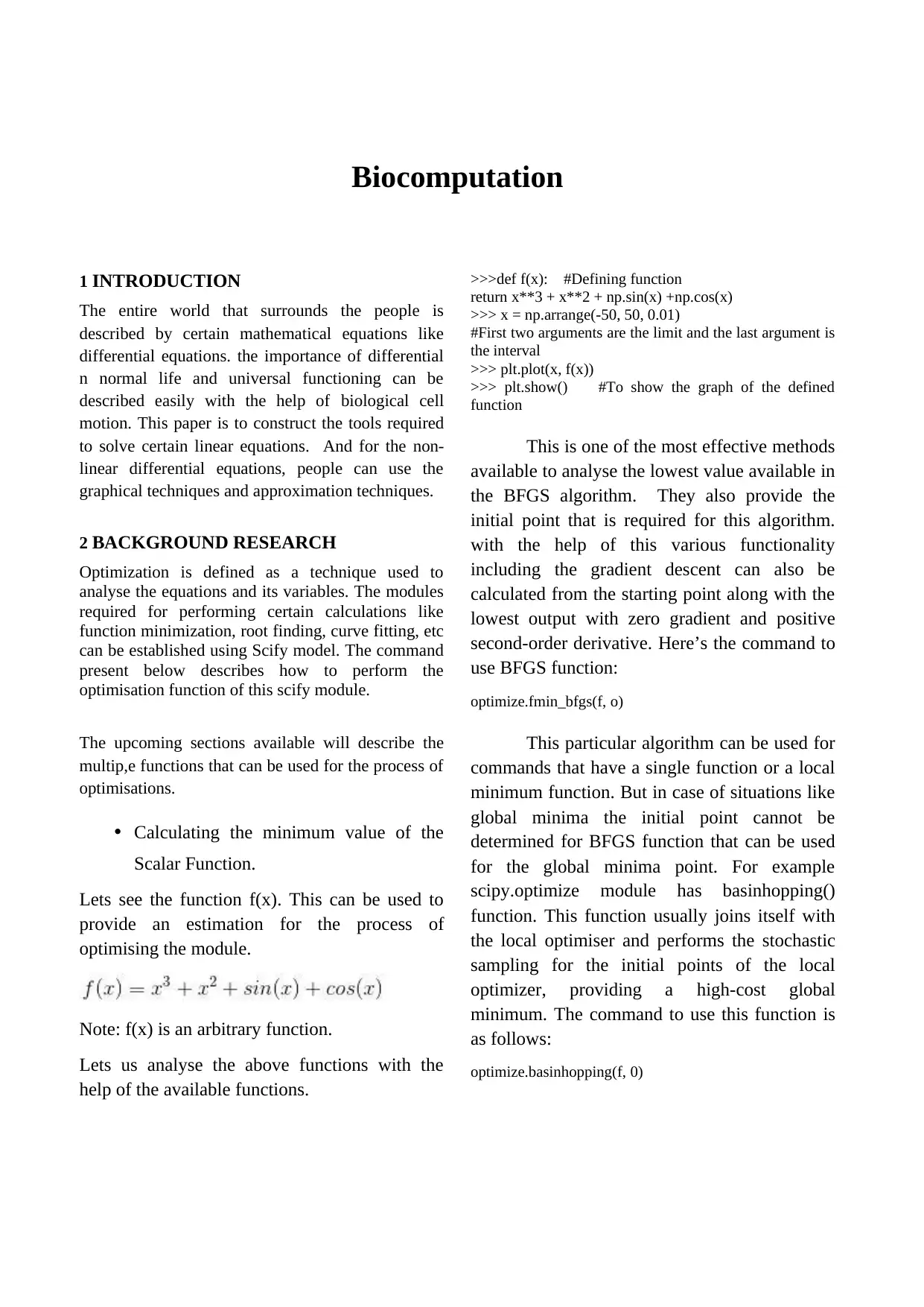
Lets see the function f(x). This can be used to
provide an estimation for the process of
optimising the module.
Note: f(x) is an arbitrary function.
Lets us analyse the above functions with the
help of the available functions.
>>>def f(x): #Defining function
return x**3 + x**2 + np.sin(x) +np.cos(x)
>>> x = np.arrange(-50, 50, 0.01)
#First two arguments are the limit and the last argument is
the interval
>>> plt.plot(x, f(x))
>>> plt.show() #To show the graph of the defined
function
This is one of the most effective methods
available to analyse the lowest value available in
the BFGS algorithm. They also provide the
initial point that is required for this algorithm.
with the help of this various functionality
including the gradient descent can also be
calculated from the starting point along with the
lowest output with zero gradient and positive
second-order derivative. Here’s the command to
use BFGS function:
optimize.fmin_bfgs(f, o)
This particular algorithm can be used for
commands that have a single function or a local
minimum function. But in case of situations like
global minima the initial point cannot be
determined for BFGS function that can be used
for the global minima point. For example
scipy.optimize module has basinhopping()
function. This function usually joins itself with
the local optimiser and performs the stochastic
sampling for the initial points of the local
optimizer, providing a high-cost global
minimum. The command to use this function is
as follows:
optimize.basinhopping(f, 0)

Crossover schemas
• Binomial (bin): This is nothing but the
cross value function that is obtained due
to the various binomial experiments.
fear the probability is considered as p-
value can be easily changed the help of
the mutant vector.
• Exponential (exp): This is generally
considered as a cross over performance
that is available in two different points
and these points can be easily chosen
with the help of vectors n. (between the
two locations) are obtained from the
mutant vector.
By providing multiple DE variants, these type
of variants can be easily Grouped together such
as rand/2/exp, best/1/exp, rand/2/bin and so on.
To perform a co bined ruling there is no
particular techniques available. So by choosing
the best variations and parameters we can use
the mutation factor, crossover probability,
population size for providing the solution to the
problem.
3 EXPERIMENTATION
Evaluation
The upcoming step is to use a linear
transformation technology for transforming the
components from [0, 1] to [min, max]. This
technique is needed for analysisng the value of
every vector along with the function fobj:
>>> pop_denorm = min_b + pop * diff
>>> pop_denorm
Here by using the the firs 10 vectors we can
perform the analysis with the help of the fobj
funtion despite their randomness and
functionality which are way better than the
other options available. (have a lower f(x)
). Let’s evaluate them:
>>> for ind in pop_denorm:
>>> print(ind, fobj(ind))
[-4.06 -4.89 -1. -2.87] 12.3984504837
[-4.57 3.69 0.19 -4.95] 14.7767132816
[ 4.58 2.78 1.51 -3.31] 10.4889711137
[-2.83 3.27 -2.72 3.43] 9.44800715266
[ 3. -0.68 -4.43 -0.57] 7.34888318457
[ 4.47 4.92 4.27 -1.05] 15.8691538075
[ 1.36 4.74 3.19 -4.37] 13.4024093959
[-0.89 -4.67 3.85 -2.61] 11.0571791104
[ 3.76 -2.14 -3.53 -4.06] 11.9129095178
[-3.67 -3.14 -3.34 -3.06] 10.9544056745
After the detailled analysis it is found that cerain
random vectors can be used. some vectors
available are x=[ 3., -0.68, -4.43, -0.57] is the
best of the population, with a f(x)=7.34
, So inorder to obtain a perfect result the value
should be approximate with the value we
require. The evaluation is done with the help of
L. 9 and stored as other variable fitness.
3.1 Function 1
f(x) = x2,
Where x is an integer in the range 0-255,
i.e., 0≤ x ≤ 255
Algorithm :
res = list(de(lambda x: sum(x**2)/len(x), [(-100,
100)] * 32, its=3000))
x,f =zip(*res)
fobj: f(x) function to optimize. Can be a function
defined with a def or a lambda expression. For
example, suppose we want to minimize the function
f(x)=∑nix2i/n
. If x is a numpy array, our fobj can be defined
as:
fobj = lambda x: sum(x**2)/len(x), [(-100, 100)] *
32, its=3000

If we define x as a list, we should define our
objective function in this way:
def fobj(x):
value = 0
for i in range(len(x)):
value += x[i]**2
return value / len(x)
print(result[-1])
(array([ 1.43231366, 4.83555112, 0.29051824,
2.94836318, 2.02918578,
-2.60703144, 0.76783095, -1.66057484,
0.42346029, -1.36945634,
-0.01227915, -3.38498397, -1.76757209,
3.16294878, 5.96335235,
3.51911452, 1.24422323, 2.9985505 , -0.13640705,
0.47221648,
0.42467349, 0.26045357, 1.20885682, -1.6256121 ,
2.21449962,
-0.23379811, 2.20160374, -1.1396289 , -0.72875512,
-3.46034836,
-5.84519163, 2.66791339]), 6.3464570348900136)
Here the best value for f(x) was 6.346, but we were
not able to get the best solution for the f(0,…,0)=0.
Why? DE does not provide the best solution for the
global minimum function. For that, we require
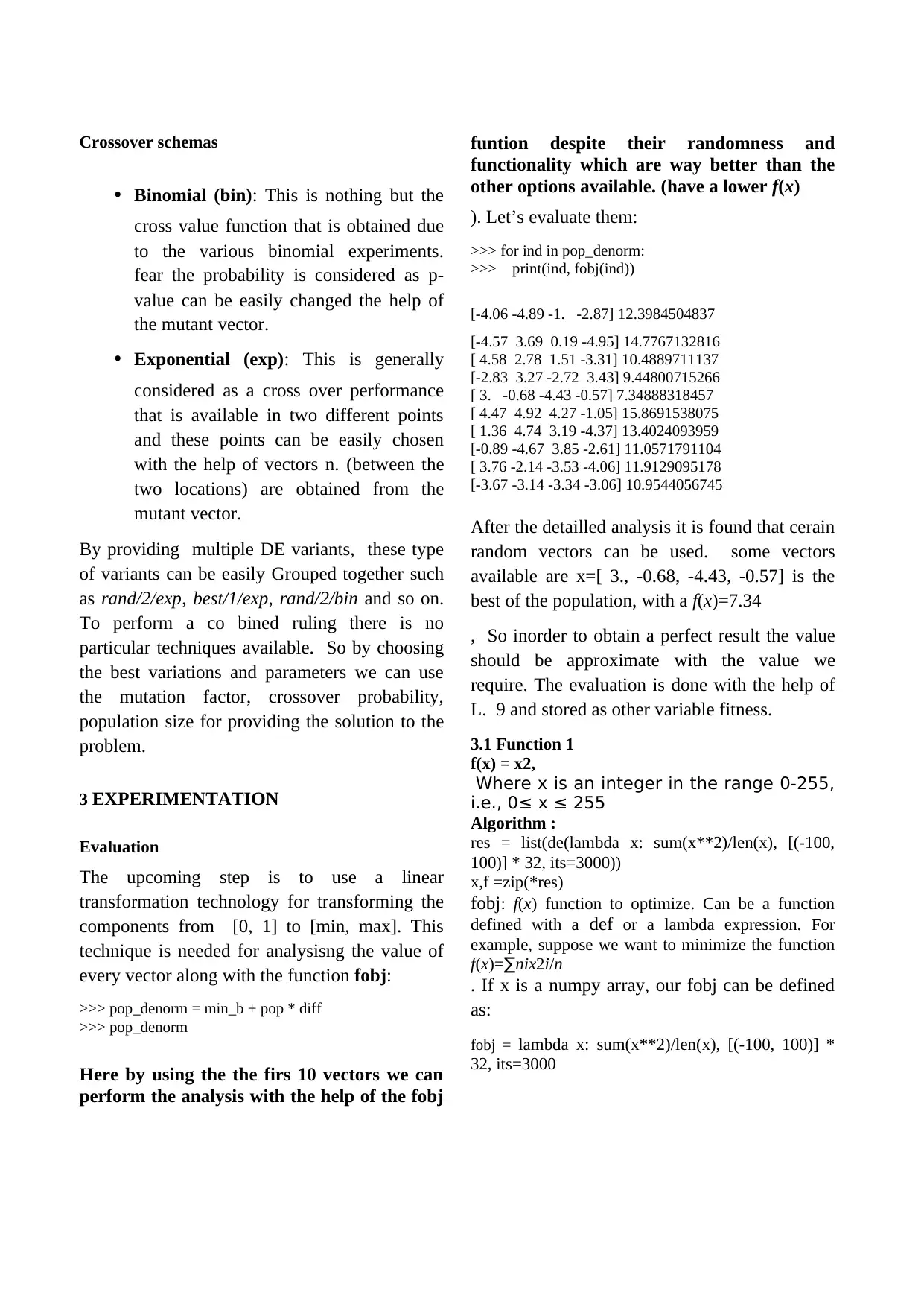
Successive steps to perform as per Fig. 1. In order to
obtain a perfect complex function, we need a number
of iterations. But in order to solve the convergence
of the algorithm in accordance with the
dimensionality of a function the difficulty of finding
the optimal solution increases exponentially with the
number of dimensions (parameters). This is also
known as “curse of dimensionality”. So if we want
to find the lowest value of a 2D function in terms of
binary values There are only two values available.
They include the worst-case scenario of 22=4
combinations of values: f(0,0), f(0,1), f(1,0) and
f(1,1). But if we have 32 parameters, we would need
to evaluate the function for a total of 232 =
4,294,967,296 possible combinations in the worst
case (the size of the search space grows
exponentially). Hence this operation is much more
easier than the values available and the any
metaheuristic algorithm like DE would need many
more iterations to find a good approximation.
Figure 1: Initial performance on dataset 1.
3.2 Function 2
f(x,y) = 0.26.( x2 + y2) – 0.48.x.y
Where -15 ≤ x,y ≤ 15
>>>print(result[-1])
(array([ 0.00648831, -0.00093694, -0.00205017,
0.00136862, -0.00722833,
-0.00138284, 0.00323691, 0.0040672 , -0.0060339 ,
0.00631543,
-0.01132894, 0.00020696, 0.00020962, -
0.00063984, -0.00877504,
-0.00227608, -0.00101973, 0.00087068,
0.00243963, 0.01391991,
-0.00894368, 0.00035751, 0.00151198,
0.00310393, 0.00219394,
0.01290131, -0.00029911, 0.00343577, -
0.00032941, 0.00021377,
-0.01015071, 0.00389961]), 3.1645278699373536e-
05)
Now we gained a perfect solution that is nearly equal
or close to 0. Here we need only a very few number
of iteration values for a perfect approximisation
which is not possible in complex values. They need
more number of iteration values to perform the
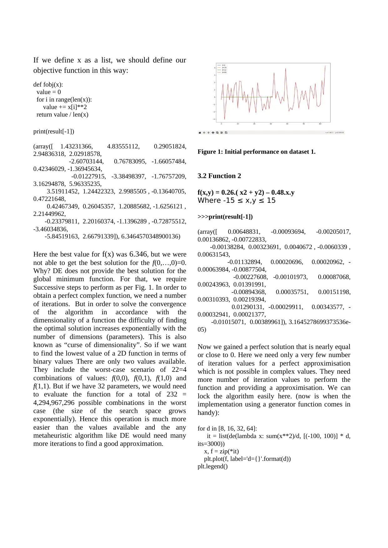
function and providing a approximisation. We can
lock the algorithm easily here. (now is when the
implementation using a generator function comes in
handy):
for d in [8, 16, 32, 64]:
it = list(de(lambda x: sum(x**2)/d, [(-100, 100)] * d,
its=3000))
x, f = zip(*it)
plt.plot(f, label='d={}'.format(d))
plt.legend()

Figure 2: Initial performance on dataset 2.
3.3 Function 3
f(x) = 10n +  xi 2– 10.cos(2pi.xi)
Where -5.12 ≤ xi ≤ 5.12, and use
n=10, 20
>>>print(result[-1])
[-4.06 -4.89 -1. -2.87] 12.3984504837
[-4.57 3.69 0.19 -4.95] 14.7767132816
[ 4.58 2.78 1.51 -3.31] 10.4889711137
[-2.83 3.27 -2.72 3.43] 9.44800715266
[ 3. -0.68 -4.43 -0.57] 7.34888318457
[ 4.47 4.92 4.27 -1.05] 15.8691538075
[ 1.36 4.74 3.19 -4.37] 13.4024093959
[-0.89 -4.67 3.85 -2.61] 11.0571791104
[ 3.76 -2.14 -3.53 -4.06] 11.9129095178
[-3.67 -3.14 -3.34 -3.06] 10.9544056745
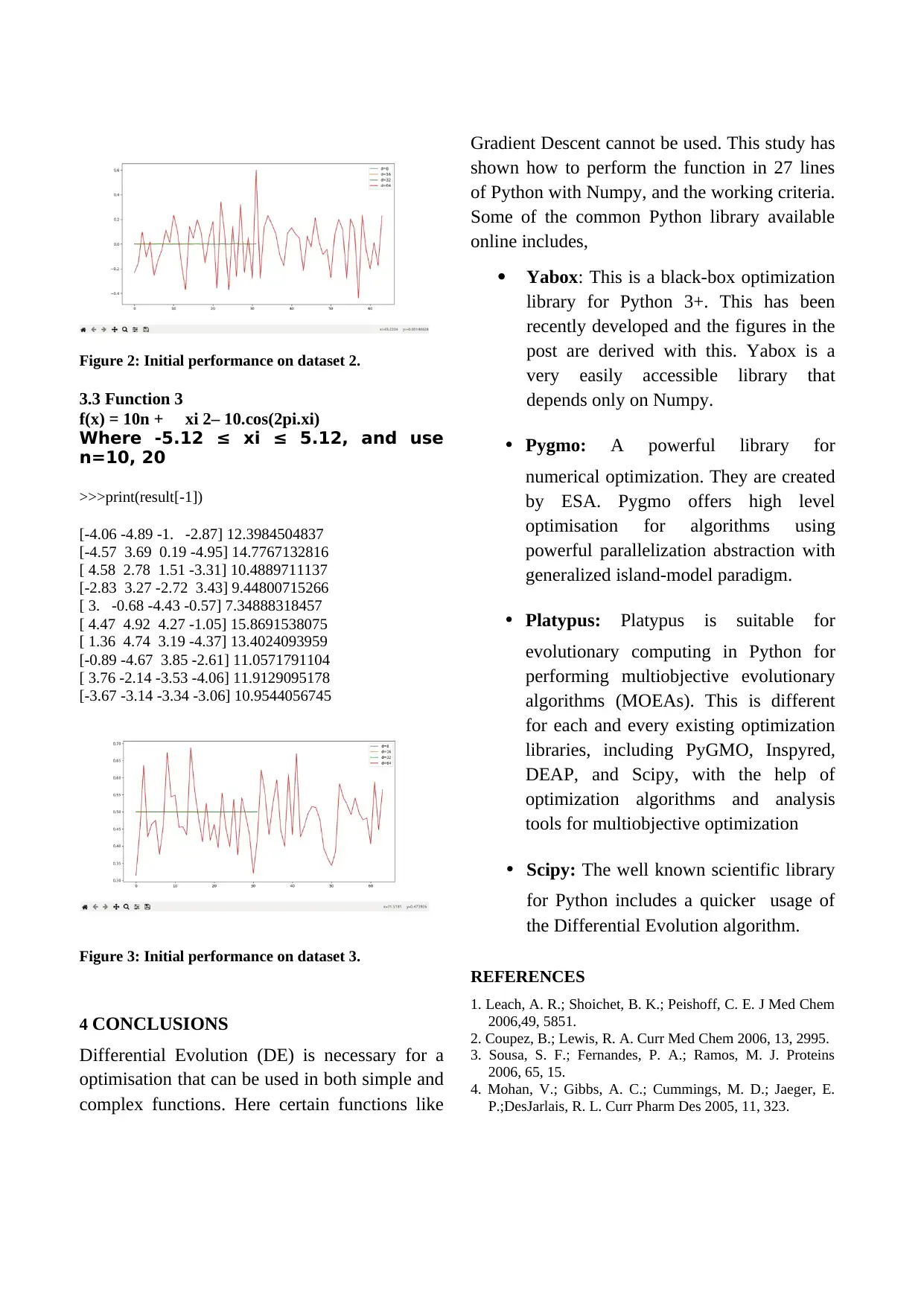
Figure 3: Initial performance on dataset 3.
4 CONCLUSIONS
Differential Evolution (DE) is necessary for a
optimisation that can be used in both simple and
complex functions. Here certain functions like
Gradient Descent cannot be used. This study has
shown how to perform the function in 27 lines
of Python with Numpy, and the working criteria.
Some of the common Python library available
online includes,
 Yabox: This is a black-box optimization
library for Python 3+. This has been
recently developed and the figures in the
post are derived with this. Yabox is a
very easily accessible library that
depends only on Numpy.
• Pygmo: A powerful library for
numerical optimization. They are created
by ESA. Pygmo offers high level
optimisation for algorithms using
powerful parallelization abstraction with
generalized island-model paradigm.
• Platypus: Platypus is suitable for
evolutionary computing in Python for
performing multiobjective evolutionary
algorithms (MOEAs). This is different
for each and every existing optimization
libraries, including PyGMO, Inspyred,
DEAP, and Scipy, with the help of
optimization algorithms and analysis
tools for multiobjective optimization
• Scipy: The well known scientific library
for Python includes a quicker usage of
the Differential Evolution algorithm.
REFERENCES
1. Leach, A. R.; Shoichet, B. K.; Peishoff, C. E. J Med Chem
2006,49, 5851.
2. Coupez, B.; Lewis, R. A. Curr Med Chem 2006, 13, 2995.
3. Sousa, S. F.; Fernandes, P. A.; Ramos, M. J. Proteins
2006, 65, 15.
4. Mohan, V.; Gibbs, A. C.; Cummings, M. D.; Jaeger, E.
P.;DesJarlais, R. L. Curr Pharm Des 2005, 11, 323.

5. Kitchen, D. B.; Decornez, H.; Furr, J. R.; Bajorath, J. Nat
Rev DrugDiscov 2004, 3, 935.
6. Brooijmans, N.; Kuntz, I. D. Annu Rev Biophys Biomol
Struct2003, 32, 335.
7. Taylor, R. D.; Jewsbury, P. J.; Essex, J. W. J Comput
Aided MolDesign 2002, 16, 151.
8. Halperin, I.; Ma, B.; Wolfson, H.; Nussinov, R. Proteins:
StructFunct Genet 2002, 47, 409.
9. Morris, G. M.; Goodsell, D. S.; Halliday, R. S.; Huey, R.;
Hart, W.E.; Belew, R. K.; Olson, A. J. J Comput Chem
1998, 19, 1639.
10. Goodsell, D. S.; Olson, A. J. Proteins: Struct Funct Genet
1990, 8,195.